pygimli.meshtools#
Mesh generation and modification.
Note
Although we discriminate here between grids (structured meshes) and meshes (unstructured), both objects are treated the same internally.
Overview#
Functions
|
Append Boundary to a given mesh. |
|
Return a copy of grid surrounded by a boundary grid. |
|
Return a copy of mesh surrounded by a tetrahedron mesh as boundary. |
|
Add a triangle mesh boundary to a given mesh. |
|
Convert cell data to boundary data. |
|
Convert cell data to node data. |
|
Check mesh for consistency. |
|
Convert mesh from foreign formats. |
|
Converts instance of a hdf5 mesh to a GIMLI::Mesh. |
|
Convert mesh from meshio object. |
|
Create simple circle polygon. |
|
Create cube PLC as geometrie definition. |
|
Create PLC of a cylinder. |
|
Create coplanar PLC from a 2d mesh or PLC. |
|
Create grid style mesh. |
|
Create a 2D pie shaped grid (segment from annulus or cirlce). |
|
Create simple line polygon. |
|
Create a mesh for a given PLC or point list. |
|
Generate simple one dimensional mesh with nodes at position in RVector pos. |
|
Generate 1D block model of thicknesses and properties |
|
Generate simple two dimensional mesh with nodes at position in RVector x and y. |
|
Generate simple three dimensional mesh with nodes at position in RVector x and y. |
|
Create a new 2D triangular mesh from the boundaries of mesh. |
|
API change here . |
|
Create parameter mesh from list of sensor positions. |
|
Create a grid-style mesh for an inversion parameter mesh. |
|
Create a geometry (PLC) for an inversion parameter mesh. |
|
Create a geometry (PLC) for an 3D inversion parameter mesh. |
|
Create surface mesh for an 3D inversion parameter mesh. |
|
Create a polygon from a list of vertices. |
|
Create rectangle polygon. |
|
Create sphere PLC as geometrie definition. |
|
Convert a 2D mesh into a 3D surface mesh. |
|
Create simple rectangular 2D or 3D world. |
|
Exports Gimli mesh in HDF5 format suitable for Fenics. |
|
Writes given GIMLI::Mesh in a hdf5 format file. |
|
Export a piece-wise linear complex (PLC) to a .poly file (2D or 3D). |
|
Write STL surface mesh and returns a GIMLI::Mesh. |
|
Extract slice from 3D mesh as triangle mesh. |
|
Extract 2d mesh from the upper surface of a 3D mesh. |
|
Create 3D body by extruding a closed 2D poly into z direction. |
|
Extrude mesh to a higher dimension. |
|
Prolongate empty cell values to complete cell attributes. |
|
Convert subsurface object to pygimli mesh. |
|
Interpolate different kind of data. |
|
Interpolate along curve. |
|
Little syntactic sugar to merge. |
|
Merge two meshes into one new mesh and return the combined mesh. |
|
Merge several meshes into one new mesh and return the new mesh. |
|
Merge multiply polygons. |
|
Merge a list of 3D PLC into one. |
|
Convert node data to boundary data. |
|
Convert node data to cell data. |
|
Return the quality of a given triangular mesh. |
|
Reads FEniCS mesh from file format .h5 and returns a GIMLI::Mesh. |
|
Read Gmsh ASCII file and return instance of GIMLI::Mesh class. |
|
Function for loading a mesh from HDF5 file format. |
|
Import mesh from Hydrus2D. |
|
Import mesh from Hydrus3D. |
|
Generic mesh read using meshio. |
|
Read in a piece-wise linear complex object (PLC) from .poly file. |
|
Read STL surface mesh and returns a GIMLI::Mesh. |
|
Read and convert a mesh from the basic Tetgen output. |
|
Read Triangle [Shewchuk, 1996] mesh. |
|
Refine mesh of hexahedra into a mesh of tetrahedra. |
|
Refine mesh of quadrangles into a mesh of triangle cells. |
|
Create a mesh from a PLC by system-calling Tetgen. |
|
Interpolate 2D tape measured topography to 2D Cartesian coordinates. |
|
Create a subsurface object from pygimli mesh. |
Functions#
- pygimli.meshtools.appendBoundary(mesh, **kwargs)[source]#
Append Boundary to a given mesh.
Syntactic sugar for
pygimli.meshtools.appendTriangleBoundaryandpygimli.meshtools.appendTetrahedronBoundary.- Parameters:
mesh (GIMLI::Mesh) – “2d or 3d Mesh to which the boundary will be appended.
:keyword **kwargs forwarded to
pygimli.meshtools.appendTriangleBoundary: :keyword orpygimli.meshtools.appendTetrahedronBoundary.:- Returns:
A new 2D or 3D mesh containing the original mesh and a boundary around.
- Return type:
- pygimli.meshtools.appendBoundaryGrid(grid, xbound=None, ybound=None, zbound=None, marker=1, isSubSurface=True, **kwargs)[source]#
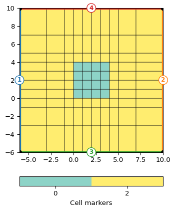
Return a copy of grid surrounded by a boundary grid.
Note, the input grid needs to be a 2d or 3d grid with quad/hex cells.
- Parameters:
grid (GIMLI::Mesh) – 2D or 3D Mesh that must contain structured quads or hex cells
xbound (iterable of type float [None]) – Needed for 2D or 3D grid prolongation and will be added on the left side in opposit order and on the right side in normal order.
ybound (iterable of type float [None]) – Needed for 2D or 3D grid prolongation and will be added (2D bottom, 3D front) in opposit order and (2D top, 3D back) in normal order.
zbound (iterable of type float [None]) – Needed for 3D grid prolongation and will be added the bottom side in opposite order on the top side in normal order.
marker (int [1]) – Cellmarker for the cells in the boundary region
isSubSurface (boolean, optional) – Apply boundary conditions suitable for geo-simulaion and prolongate mesh to the surface if necessary, e.i., no boundary on top of the grid.
Examples
>>> import pygimli as pg
>>> import pygimli.meshtools as mt
>>> grid = mt.createGrid(5,5)
...
>>> g1 = mt.appendBoundaryGrid(grid,
...                            xbound=[1, 3, 6],
...                            ybound=[1, 3, 6],
...                            marker=2,
...                            isSubSurface=False)
>>> ax,_ = pg.show(g1, markers=True, showMesh=True)
>>> grid = mt.createGrid(5,5,5)
...
>>> g2 = mt.appendBoundaryGrid(grid,
...                            xbound=[1, 3, 6],
...                            ybound=[1, 3, 6],
...                            zbound=[1, 3, 6],
...                            marker=2,
...                            isSubSurface=False)
>>> ax, _ = pg.show(g2, g2.cellMarkers(), showMesh=True,
...                 filter={'clip':{}});
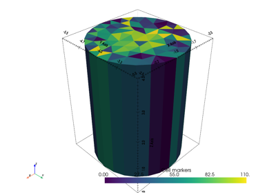
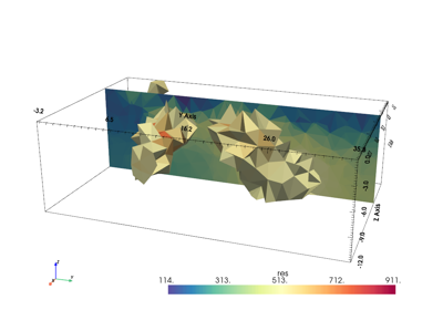
- pygimli.meshtools.appendTetrahedronBoundary(mesh, xbound=10, ybound=10, zbound=10, marker=1, isSubSurface=True, **kwargs)[source]#
Return a copy of mesh surrounded by a tetrahedron mesh as boundary.
Returns a new mesh that contains a tetrahedron mesh box around a given mesh suitable for geo-simulation (surface boundary with marker = -1 at top and marker = -2 in the inner subsurface). The old boundary marker from mesh will be preserved, except for marker == -2 which will be switched to 2 as we assume -2 is the world marker for outer boundaries in the subsurface.
Note
This method will only work stable if the mesh generator (Tetgen) preserves all input boundaries. This will lead to bad quality meshes for the boundary region so its a good idea to play with the addNodes keword argument to manually refine the newly created outer boundaries.
If the input mesh consists of hexahedrons a small inconsistency will arise because a quad boundary element will be split by 2 triangle boundaries from the boundary tetrahedrons. The effect of this hanging edges are unclear, also createNeighbourInfos may fail. We need to implement/test pyramid cells to handle this.
- Parameters:
mesh (GIMLI::Mesh) – 3D Mesh to which the tetrahedron boundary should be appended.
xbound (float [10]) – Horizontal prolongation distance in meter at x-direction. Need to be >= 0.
ybound (float [10]) – Horizonal prolongation distance in meter at y-direction. Need to be greater 0.
zbound (float [10]) – Vertical prolongation distance in meter at z-direction (>0).
marker (int, optional) – Marker of new cells.
addNodes (float, optional) – Triangle quality.
isSubSurface (boolean, optional) – Apply boundary conditions suitable for geo-simulaion and prolongate mesh to the surface if necessary.
verbose (boolean, optional) – Be verbose.
- Returns:
A new 3D mesh containing the original mesh and a boundary arround.
- Return type:
Examples
>>> import pygimli as pg
>>> import pygimli.meshtools as mt
>>> grid = mt.createGrid(5,5,5)
...
>>> mesh = mt.appendBoundary(grid, xbound=5, ybound=5, zbound=5,
...                          isSubSurface=False)
>>> ax, _ = pg.show(mesh, mesh.cellMarkers(), showMesh=True,
...                 filter={'clip':{}})
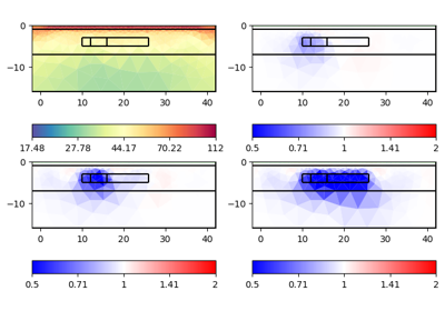
- pygimli.meshtools.appendTriangleBoundary(mesh, xbound=10, ybound=10, marker=1, isSubSurface=True, **kwargs)[source]#
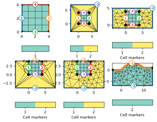
Add a triangle mesh boundary to a given mesh.
Returns a new mesh that contains a triangulated box around a given mesh suitable for geo-simulation (surface boundary with marker == -1 at the top and marker == -2 in the inner subsurface). The old boundary marker from the input mesh are preserved, except for marker == -2 which will be changed to +2 as we assume marker == -2 is the world marker for outer boundaries in the subsurface.
Note, this all will only work stable if the mesh generator (triangle) preserve all input boundaries. However this will lead to bad quality meshes for the boundary region so its a good idea to play with the addNodes keyword argument to manually refine the newly created outer boundaries.
- Parameters:
mesh (GIMLI::Mesh) – Mesh to which the triangle boundary should be appended.
xbound (float, optional) – Absolute horizontal prolongation distance. Need to be greater 2.
ybound (float, optional) – Absolute vertical prolongation distance.
marker (int, optional) – Marker of new cells.
isSubSurface (boolean [True]) – Apply boundary conditions suitable for geo-simulation and prolongate mesh to the surface if necessary.
- Keyword Arguments:
pg.createMesh (** kargs forwarded to)
quality (float, optional) – Triangle quality.
area (float, optional) – Triangle max size within the boundary.
smooth (boolean, optional) – Apply mesh smoothing.
addNodes (int[5], iterable) – Add additional nodes on the outer boundaries. Or for each boundary if given 5 values (isSubsurface=True) or 4 for isSubsurface=False
- Returns:
A new 2D mesh containing the original mesh and a boundary arround.
- Return type:
Examples
>>> import matplotlib.pyplot as plt
>>> import pygimli as pg
>>> from pygimli.viewer.mpl import drawMesh, drawModel
>>> import pygimli.meshtools as mt
>>> inner = pg.createGrid(range(5), range(5), marker=1)
>>> fig, axs = plt.subplots(2,3)
>>> ax, _ = pg.show(inner, markers=True, showBoundaries=True, showMesh=True, ax=axs[0][0])
>>> m = mt.appendTriangleBoundary(inner, xbound=3, ybound=3, marker=2, addNodes=0, isSubSurface=False)
>>> ax, _ = pg.show(m, markers=True, showBoundaries=True, showMesh=True, ax=axs[0][1])
>>> m = mt.appendTriangleBoundary(inner, xbound=4, ybound=1, marker=2, addNodes=5, isSubSurface=False)
>>> ax, _ = pg.show(m, markers=True, showBoundaries=True, showMesh=True, ax=axs[0][2])
>>> m = mt.appendTriangleBoundary(inner, xbound=4, ybound=4, marker=2, addNodes=0, isSubSurface=True)
>>> ax, _ = pg.show(m, markers=True, showBoundaries=True, showMesh=True, ax=axs[1][0])
>>> m = mt.appendTriangleBoundary(inner, xbound=4, ybound=4, marker=2, addNodes=5, isSubSurface=True)
>>> ax, _ = pg.show(m, markers=True, showBoundaries=True, showMesh=True, ax=axs[1][1])
>>> surf = mt.createPolygon([[0, 0],[5, 3], [10, 1]], boundaryMarker=-1, addNodes=5, interpolate='spline')
>>> m = mt.appendTriangleBoundary(surf, xbound=4, ybound=4, marker=2, addNodes=5, isSubSurface=True)
>>> ax, _ = pg.show(m, markers=True, showBoundaries=True, showMesh=True, ax=axs[1][2])
Examples using pygimli.meshtools.appendTriangleBoundary
- pygimli.meshtools.cellDataToNodeData(mesh, data, style='mean')[source]#
Convert cell data to node data.
Convert cell data to node data via non-weighted averaging (mean) of common cell data.
- Parameters:
mesh (GIMLI::Mesh) – 2D or 3D GIMLi mesh
data (iterable [float]) – Data of len mesh.cellCount(). TODO complex, R3Vector, ndarray
style (str ['mean']) – Interpolation style. * ‘mean’ : non-weighted averaging TODO harmonic averaging TODO weighted averaging (mean, harmonic) TODO interpolation via cell centered mesh
Examples
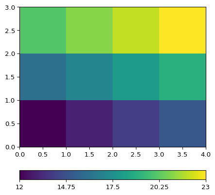
>>> import pygimli as pg
>>> grid = pg.createGrid(x=(1,2,3),y=(1,2,3))
>>> celldata = np.array([1, 2, 3, 4])
>>> nodedata = pg.meshtools.cellDataToNodeData(grid, celldata)
>>> print(nodedata.array())
[1.  1.5 2.  2.  2.5 3.  3.  3.5 4. ]
Examples using pygimli.meshtools.cellDataToNodeData
- pygimli.meshtools.checkMeshConsistency(mesh)[source]#
Check mesh for consistency.
Checks if all nodes are used in cells.
Checks if all outer boundaries have only a left cell.
Checks if all outer boundaries normal vector points outward.
- Parameters:
mesh (GIMLI::Mesh) – Mesh to be checked.
- Returns:
True if mesh is consistent, False otherwise.
- Return type:
bool
- pygimli.meshtools.convertHDF5Mesh(h5Mesh, group='mesh', indices='cell_indices', pos='coordinates', cells='topology', marker='values', marker_default=0, dimension=3, verbose=True, useFenicsIndices=False)[source]#
Converts instance of a hdf5 mesh to a GIMLI::Mesh.
For full documentation please see
pygimli:meshtools:readHDF5Mesh.
- pygimli.meshtools.convertMeshioMesh(mesh, verbose=False)[source]#
Convert mesh from meshio object.
See https://pypi.org/project/meshio/1.8.9/
- TODO
test for 3D mesh
test and improve if neeeded
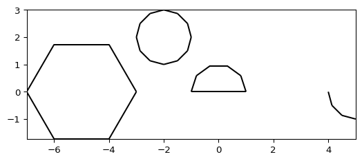
- pygimli.meshtools.createCircle(pos=None, radius=1, nSegments=12, start=0, end=6.283185307179586, **kwargs)[source]#
Create simple circle polygon.
Create simple circle polygon with given attributes.
- Parameters:
pos ([x, y] [[0.0, 0.0]]) – Center position
radius (float | [a,b] [1]) – radius or halfaxes of the circle
nSegments (int [12]) – Discrete amount of segments for the circle.
start (double [0]) – Starting angle in radians
end (double [2*pi]) – Ending angle in radians
**kwargs –
- marker: int [1]
Marker for the resulting triangle cells after mesh generation
- markerPositionfloats [x, y] [0.0, 0.0]
Position of the marker (works for both regions and holes)
- area: float [0]
Maximum cell size for resulting triangles after mesh generation
- isHole: bool [False]
The polygon will become a hole instead of a triangulation
- boundaryMarker: int [1]
Marker for the resulting boundary edges
- leftDirection: bool [True]
Rotational direction
- isClosed: bool [True]
Add closing edge between last and first node.
- Returns:
poly – The resulting polygon is a GIMLI::Mesh.
- Return type:
Examples
>>>  # no need to import matplotlib. pygimli's show does
>>> import math
>>> import pygimli as pg
>>> from pygimli.viewer.mpl import drawMesh
>>> import pygimli.meshtools as mt
>>> c0 = mt.createCircle(pos=(-5.0, 0.0), radius=2, nSegments=6)
>>> c1 = mt.createCircle(pos=(-2.0, 2.0), radius=1, area=0.01, marker=2)
>>> c2 = mt.createCircle(pos=(0.0, 0.0), nSegments=5, start=0, end=math.pi)
>>> c3 = mt.createCircle(pos=(5.0, 0.0), nSegments=3, start=math.pi,
...                      end=1.5*math.pi, isClosed=False)
>>> plc = mt.mergePLC([c0, c1, c2, c3])
>>> fig, ax = pg.plt.subplots()
>>> drawMesh(ax, plc, fillRegion=False)
>>> pg.wait()
Examples using pygimli.meshtools.createCircle
- pygimli.meshtools.createCube(size=None, pos=None, start=None, end=None, rot=None, boundaryMarker=0, **kwargs)[source]#
Create cube PLC as geometrie definition.
Create cube PLC as geometrie definition. You can either give size and center position or start and end position.
- Parameters:
size ([x, y, z]) – x, y, and z-size of the cube. Default = [1.0, 1.0, 1.0] in m
pos ([x, y, z]) – The center position, default is at the origin.
start ([x, y, z]) – Left Front Bottom corner.
end ([x, y, z]) – Right Back Top corner.
rot (pg.Pos [None]) – Rotate on the center.
boundaryMarker (int[0]) – Boundary marker for the resulting faces.
kwargs (**) – Marker related arguments: See
pygimli.meshtools.polytools.setPolyRegionMarker
Examples
>>> import pygimli.meshtools as mt
>>> cube = mt.createCube()
>>> print(cube)
Mesh: Nodes: 8 Cells: 0 Boundaries: 6
>>> cube = mt.createCube([10, 10, 1])
>>> print(cube.bb())
[RVector3: (-5.0, -5.0, -0.5), RVector3: (5.0, 5.0, 0.5)]
>>> cube = mt.createCube([10, 10, 1], pos=[-4.0, 0.0, 0.0])
>>> print(pg.center(cube.positions()))
RVector3: (-4.0, 0.0, 0.0)
- Returns:
poly – The resulting polygon is a GIMLI::Mesh.
- Return type:
Examples using pygimli.meshtools.createCube
- pygimli.meshtools.createCylinder(radius=1, height=1, nSegments=8, pos=None, rot=None, boundaryMarker=0, **kwargs)[source]#
Create PLC of a cylinder.
Out of core wrapper for dcfemlib::polytools.
Note, there is a bug in the old polytools which ignores the area settings for marker == 0.
- Parameters:
radius (float) – Radius of the cylinder.
height (float) – Height of the cylinder
nSegments (int [8]) – Number of segments of the cylinder.
pos (pg.Pos [None]) – The center position, default is at the origin.
- Keyword Arguments:
kwargs (**) – Marker related arguments: See
pygimli.meshtools.polytools.setPolyRegionMarker- Returns:
poly – The resulting polygon is a GIMLI::Mesh.
- Return type:
- pygimli.meshtools.createFacet(mesh, boundaryMarker=None)[source]#
Create coplanar PLC from a 2d mesh or PLC.
- Parameters:
mesh (pg.Mesh) – 2D mesh or PLC to be converted to a 3D facet
boundaryMarker (int) – boundary marker for the facet, otherwise taken from 2d region markers
- Returns:
plc – plc of the created facet
- Return type:
pyGIMLi mesh
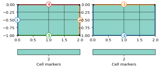
- pygimli.meshtools.createGrid(x=None, y=None, z=None, **kwargs)[source]#
Create grid style mesh.
Generate simple grid with defined node positions for each dimension. The resulting grid depends on the amount of given coordinate arguments and consists out of edges (1D - x), quads (2D- x and y), or hexahedrons(3D- x, y, and z). For grids with world boundary markers (-1 surface and -2 subsurface) the y or z array need to be in increasing order.
- Parameters:
kwargs –
- x: array
x-coordinates for all Nodes (1D, 2D, 3D)
- y: array
y-coordinates for all Nodes (2D, 3D)
- z: array
z-coordinates for all Nodes (3D)
- marker: int = 0
Marker for resulting cells.
- worldBoundaryMarkerbool = False
Boundaries are enumerated with world marker, i.e., Top = -1 All remaining = -2. Default markers: left=1, right=2, top=3, bottom=4, front=5, back=6
- Returns:
Either 1D, 2D or 3D mesh depending the input.
- Return type:
Examples
>>> import pygimli as pg
>>> mesh = pg.meshtools.createGrid(x=[0, 1, 1.5, 2], y=[-1, -.5, -.25, 0],
...                                marker=2)
>>> print(mesh)
Mesh: Nodes: 16 Cells: 9 Boundaries: 24
>>> fig, axs = pg.plt.subplots(1, 2)
>>> _ = pg.show(mesh, markers=True, showMesh=True, ax=axs[0])
>>> mesh = pg.meshtools.createGrid(x=[0, 1, 1.5, 2], y=[-1, -.5, -0.25, 0],
...                                worldBoundaryMarker=True, marker=2)
>>> print(mesh)
Mesh: Nodes: 16 Cells: 9 Boundaries: 24
>>> _ = pg.show(mesh, markers=True, showBoundaries=True,
...             showMesh=True, ax=axs[1])
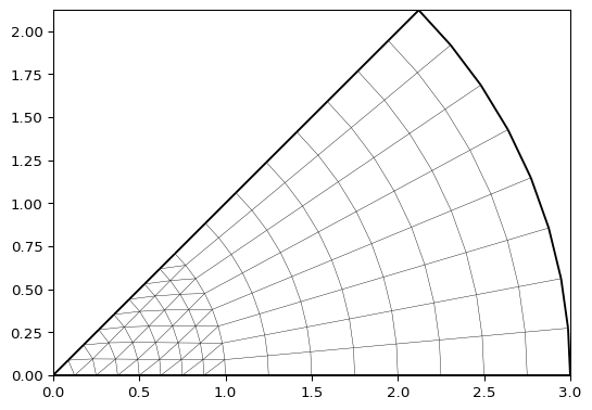
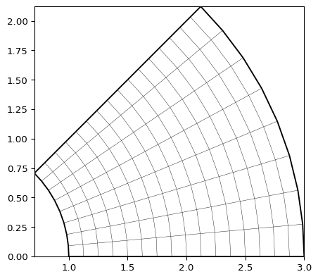
- pygimli.meshtools.createGridPieShaped(x, degree=10.0, h=2, marker=0)[source]#
Create a 2D pie shaped grid (segment from annulus or cirlce).
- Parameters:
x (array) – x-coordinates for all Nodes (2D). If you need it 3D, you can apply
pygimli.meshtools.extrudeMeshon it.degree (float [None]) – Create a pie shaped grid for a value between 0 and 90. Creates an optional inner boundary (marker=2) for a annulus with x[0] > 0. Outer boundary marker is 1. Optional h refinement. Center node is the first for circle segment.
h (int [2]) – H-Refinement for degree option.
marker (int = 0) – Marker for resulting cells.
- Returns:
mesh
- Return type:
Examples
>>> import pygimli as pg
>>> mesh = pg.meshtools.createGridPieShaped(x=[0, 1, 3], degree=45, h=3)
>>> print(mesh)
Mesh: Nodes: 117 Cells: 128 Boundaries: 244
>>> _ = pg.show(mesh)
>>> mesh = pg.meshtools.createGridPieShaped(x=[1, 2, 3], degree=45, h=3)
>>> print(mesh)
Mesh: Nodes: 153 Cells: 128 Boundaries: 280
>>> _ = pg.show(mesh)
- pygimli.meshtools.createLine(start, end, nSegments=1, **kwargs)[source]#
Create simple line polygon.
Create simple line polygon from start to end.
- Parameters:
start ([x, y]) – start position
end ([x, y]) – end position
nSegments (int) – Discrete amount of segments for the line
- Keyword Arguments:
boundaryMarker (int [1]) – Marker for the resulting boundary edges
leftDirection (bool [True]) – Rotational direction
- Returns:
poly – The resulting polygon is a GIMLI::Mesh.
- Return type:
Examples
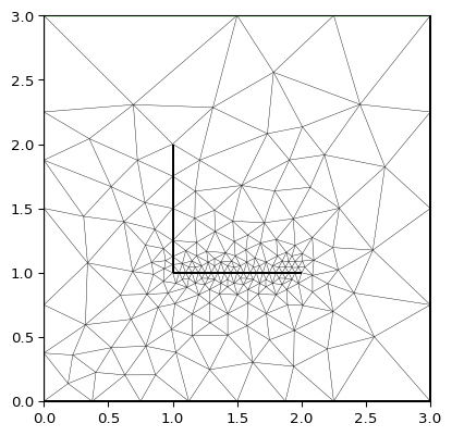
>>>  # no need to import matplotlib. pygimli's show does
>>> import pygimli as pg
>>> import pygimli.meshtools as mt
>>>
>>> w = mt.createWorld(start=[0, 0], end=[3, 3])
>>> l1 = mt.createLine(start=[1, 1], end=[1, 2], nSegments=1,
...                    leftDirection=False)
>>> l2 = mt.createLine(start=[1, 1], end=[2, 1], nSegments=20,
...                    leftDirection=True)
>>>
>>> ax, _ = pg.show(mt.createMesh([w, l1, l2,]))
>>> ax, _ = pg.show([w, l1, l2,], ax=ax, fillRegion=False)
>>> pg.wait()
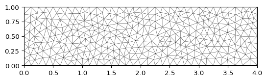
- pygimli.meshtools.createMesh(poly, quality=32, area=0.0, smooth=None, switches=None, verbose=False, **kwargs)[source]#
Create a mesh for a given PLC or point list.
The mesh is created by triangle or tetgen if the pgGIMLi support for these mesh generators is installed. A PLC needs to contain nodes and boundaries and should be valid in the sense that the boundaries are non-intersecting.
If poly is a list of coordinates, a simple Delaunay mesh with a convex hull will be created. Quality and area arguments are ignored for this case to create a mesh with one node for each coordinate position.
- Parameters:
poly (GIMLI::Mesh or list or ndarray) –
2D or 3D GIMli mesh that contains the PLC.
2D mesh needs edges
3D mesh needs a plc and tetgen as system component
List of x y pairs [[x0, y0], … ,[xN, yN]]
ndarray [x_i, y_i]
PLC or list of PLCs
quality (float) – 2D triangle quality sets a minimum angle constraint. Be careful with values above 34 degrees. 3D tetgen quality. Be careful with values below 1.12.
area (float) – Maximum element size (global). 2D maximum triangle size in m*², 3D maximum tetrahedral size in m³.
smooth (tuple) –
[smoothing algorithm, number of iterations] 0: no smoothing 1: node center 2: weighted node center
If smooth is just set to True then [1, 4] is chosen.
switches (str) – Set additional triangle command switches. https://www.cs.cmu.edu/~quake/triangle.switch.html
Args (Additional)
---------------
preserveBoundary (bool) – Preserver boundary nodes, no more nodes on boundaries.
- Returns:
mesh
- Return type:
Examples
>>> import pygimli as pg
>>> import pygimli.meshtools as mt
>>> rect = mt.createRectangle(start=[0, 0], end=[4, 1])
>>> ax, _ = pg.show(mt.createMesh(rect, quality=10))
>>> ax, _ = pg.show(mt.createMesh(rect, quality=33))
>>> ax, _ = pg.show(mt.createMesh(rect, quality=33, area=0.01))
>>> pg.wait()
Examples using pygimli.meshtools.createMesh
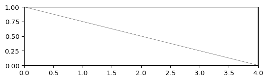
- pygimli.meshtools.createMesh1D((object)x) object :#
Generate simple one dimensional mesh with nodes at position in RVector pos.
- C++ signature :
GIMLI::Mesh createMesh1D(GIMLI::Vector<double>)
- createMesh1D( (object)nCells [, (object)nProperties=1]) -> object :
Generate simple 1D mesh with nCells cells of length 1, and nCells + 1 nodes. In case of more than one property quasi-2d mesh with regions is generated.
- C++ signature :
GIMLI::Mesh createMesh1D(unsigned long [,unsigned long=1])
- pygimli.meshtools.createMesh1DBlock((object)nLayers[, (object)nProperties=1]) object :#
Generate 1D block model of thicknesses and properties
- C++ signature :
GIMLI::Mesh createMesh1DBlock(unsigned long [,unsigned long=1])
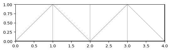
- pygimli.meshtools.createMesh2D((object)x, (object)y[, (object)markerType=0]) object :#
Generate simple two dimensional mesh with nodes at position in RVector x and y.
- C++ signature :
GIMLI::Mesh createMesh2D(GIMLI::Vector<double>,GIMLI::Vector<double> [,int=0])
- createMesh2D( (object)mesh, (object)y [, (object)frontMarker=0 [, (object)backMarker=0 [, (object)leftMarker=0 [, (object)rightMarker=0 [, (object)adjustBack=False]]]]]) -> object :
Generate a simple 2D mesh by extruding a 1D polygone into RVector y using quads. We assume a 2D mesh here consisting on nodes and edge boundaries. Nodes with marker are extruded as edges with marker or set to front- and backMarker. Edges with marker are extruded as cells with marker. All back y-coordinates are adjusted if adjustBack is set.
- C++ signature :
GIMLI::Mesh createMesh2D(GIMLI::Mesh,GIMLI::Vector<double> [,int=0 [,int=0 [,int=0 [,int=0 [,bool=False]]]]])
- createMesh2D( (object)xDim, (object)yDim [, (object)markerType=0]) -> object :
Generate simple two dimensional mesh with nRows x nCols cells with each length = 1.0
- C++ signature :
GIMLI::Mesh createMesh2D(unsigned long,unsigned long [,int=0])
Examples using pygimli.meshtools.createMesh2D
- pygimli.meshtools.createMesh3D((object)x, (object)y, (object)z[, (object)markerType=0]) object :#
Generate simple three dimensional mesh with nodes at position in RVector x and y.
- C++ signature :
GIMLI::Mesh createMesh3D(GIMLI::Vector<double>,GIMLI::Vector<double>,GIMLI::Vector<double> [,int=0])
- createMesh3D( (object)mesh, (object)z [, (object)topMarker=0 [, (object)bottomMarker=0]]) -> object :
Generate a simple three dimensional mesh by extruding a two dimensional mesh into RVector z using triangle prism or hexahedrons or both. 3D cell marker are set from 2D cell marker. The boundary marker for the side boundaries are set from edge marker in mesh. Top and bottomLayer boundary marker are set from parameter topMarker and bottomMarker.
- C++ signature :
GIMLI::Mesh createMesh3D(GIMLI::Mesh,GIMLI::Vector<double> [,int=0 [,int=0]])
- createMesh3D( (object)xDim, (object)yDim, (object)zDim [, (object)markerType=0]) -> object :
Generate simple three dimensional mesh with nx x nx x nz cells with each length = 1.0
- C++ signature :
GIMLI::Mesh createMesh3D(unsigned long,unsigned long,unsigned long [,int=0])
Examples using pygimli.meshtools.createMesh3D
- pygimli.meshtools.createMeshFromHull(mesh, fixNodes=[], **kwargs)[source]#
Create a new 2D triangular mesh from the boundaries of mesh.
- Parameters:
mesh (GIMLI::Mesh) – Input mesh.
fixNodes (iterable (int)) – Nodes (IDs) from the input mesh that should be part of the new mesh.
- Keyword Arguments:
**kwargs (dict) – Forwarded to
pygimli:meshtools:createMesh.- Returns:
mesh – Returning mesh. If fixed nodes are requested, a list of the new IDs are returned in advance.
- Return type:
GIMLI::Mesh, List of fixed nodes
- pygimli.meshtools.createParaDomain2D(*args, **kwargs)[source]#
API change here .. use createParaMeshPLC instead.
- pygimli.meshtools.createParaMesh(data, **kwargs)[source]#
Create parameter mesh from list of sensor positions.
Create parameter mesh from list of sensor positions. Uses :py:func:pygimli.meshtools.createParaMeshPLC and :py:func:pygimli.meshtools.createMesh and forwards keyword arguments.
- Parameters:
data (DataContainer) – Data container to read sensors positions from.
- Keyword Arguments:
` (Forwarded to)
- Returns:
poly
- Return type:
Examples using pygimli.meshtools.createParaMesh
- pygimli.meshtools.createParaMesh2DGrid(sensors, paraDX=1, paraDZ=1, paraDepth=0, nLayers=11, boundary=-1, paraBoundary=2, **kwargs)[source]#
Create a grid-style mesh for an inversion parameter mesh.
Create a grid-style mesh for an inversion parameter mesh. Return parameter grid for a given list of sensor positions. Uses and forwards arguments to
pygimli.meshtools.appendTriangleBoundary.- Parameters:
sensors (list of RVector3 objects or data container with sensorPositions) – Sensor positions. Must be sorted in positive x direction
paraDX (float, optional) – Horizontal distance between sensors, relative regarding sensor distance. Value must be greater than 0 otherwise 1 is assumed.
paraDZ (float, optional) – Vertical distance to the first depth layer, relative regarding sensor distance. Value must be greater than 0 otherwise 1 is assumed.
paraDepth (float, optional) – Maximum depth for parametric domain, 0 (default) means 0.4 * maximum sensor range.
nLayers (int, optional [11]) – Number of depth layers.
boundary (int, optional [-1]) – Boundary width to be appended for domain prolongation in absolute para domain width. Values lower than 0 force the boundary to be 4 times para domain width.
paraBoundary (int, optional [2]) – Offset to the parameter domain boundary in absolute sensor spacing.
- Returns:
mesh
- Return type:
Examples
>>> import pygimli as pg
>>> import matplotlib.pyplot as plt
>>>
>>> from pygimli.meshtools import createParaMesh2DGrid
>>> mesh = createParaMesh2DGrid(sensors=pg.Vector(range(10)),
...                             boundary=5, paraDX=1,
...                             paraDZ=1, paraDepth=5)
>>> ax, _ = pg.show(mesh, markers=True, showMesh=True)
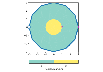
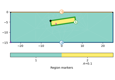
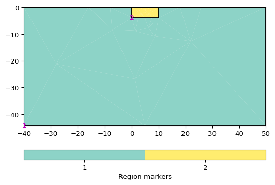
- pygimli.meshtools.createParaMeshPLC(sensors, paraDX=1, paraDepth=-1, paraBoundary=2, paraMaxCellSize=0.0, boundary=-1, boundaryMaxCellSize=0, balanceDepth=True, isClosed=False, addNodes=1, **kwargs)[source]#
Create a geometry (PLC) for an inversion parameter mesh.
Create an inversion mesh geometry (PLC) for a given list of sensor positions. Sensor positions are assumed to be on the surface and must be unique and sorted along x coordinate.
You can create a parameter mesh without sensors if you just set [xMin, xMax] as sensors.
The PLC is a GIMLI::Mesh and contain nodes, edges and two region markers, one for the parameters domain (marker=2) and a larger boundary around the outside (marker=1).
- Parameters:
sensors ([RVector3] | DataContainer with sensorPositions() | [xMin, xMax]) – Sensor positions. Must be sorted and unique in positive x direction. Depth need to be y-coordinate.
paraDX (float [1]) – Relative distance for refinement nodes between two sensors (1=none), e.g., 0.5 means 1 additional node between two neighboring sensors e.g., 0.33 means 2 additional equidistant nodes between two sensors
paraDepth (float[-1], optional) – Maximum depth in m for parametric domain. Automatic (<=0) results in 0.4 * maximum sensor span range in m
balanceDepth (bool [True]) – Equal depth for the parametric domain.
paraBoundary (float, optional) – Margin for parameter domain in absolute sensor distances. 2 (default).
paraMaxCellSize (double, optional) – Maximum cell size for parametric region in m²
boundaryMaxCellSize (double, optional) – Maximum cells size in the boundary region in m²
boundary (float, optional) – Boundary width to be appended for domain prolongation in absolute para domain width. Values lover 0 force the boundary to be 4 times para domain width.
isClosed (bool [False]) – Create a closed geometry from sensor positions. Region marker is 1. Boundary marker is -1 (homogeneous Neumann)
addNodes (int [1]) – Number of additional nodes to be added equidistant between sensors.
trapRatio (float [0]) – Form a trapezoidal shape instead of a rectangle. The value is a ratio of the total length to put inside at depth.
- Returns:
poly – Piecewise linear complex (PLC) containing nodes and edges
- Return type:
Examples
>>> # no need to import matplotlib, pygimli show does.
>>> import pygimli as pg
>>> import pygimli.meshtools as mt
>>> # Create the simplest paramesh PLC with a para box of 10 m without
>>> # sensors
>>> p = mt.createParaMeshPLC([0,10])
>>> # you can add subsurface sensors now with
>>> for z in range(1,4):
...     n = p.createNode((5,-z), -99)
>>> ax,_ = pg.show(p)
Examples using pygimli.meshtools.createParaMeshPLC
- pygimli.meshtools.createParaMeshPLC3D(sensors, paraDX=0, paraDepth=-1, paraBoundary=None, paraMaxCellSize=0.0, boundary=None, boundaryMaxCellSize=0, surfaceMeshQuality=30, surfaceMeshArea=0, addTopo=None, isClosed=False, **kwargs)[source]#
Create a geometry (PLC) for an 3D inversion parameter mesh.
- Parameters:
sensors (Sensor list or pg.DataContainer with .sensors()) – Sensor positions.
paraDX (float [1]) – Absolute distance for node refinement (0=none). Refinement node will be placed below the surface.
paraDepth (float[-1], optional) – Maximum depth in m for parametric domain. Automatic (<=0) results in 0.4 * maximum sensor span range in m. Depth is set to median sensors depth + paraDepth.
paraBoundary ([float, float] | float [1.1, 1.1]) – Margin for parameter domain in relative extend.
paraMaxCellSize (double, optional) – Maximum cell size for parametric region in m³
boundaryMaxCellSize (double, optional) – Maximum cells size in the boundary region in m³
boundary ([float, float] | float [10., 10.]) – Boundary width to be appended for domain prolongation in relative para domain size.
surfaceMeshQuality (float [30]) – Quality of the surface mesh.
surfaceMeshArea (float [0]) – Max boundary size for surface area in parametric region.
addTopo ([[x,y,z],]) – Number of additional nodes for topography.
- Returns:
poly – Piecewise linear complex (PLC) containing nodes and edges
- Return type:
Examples using pygimli.meshtools.createParaMeshPLC3D
- pygimli.meshtools.createParaMeshSurface(sensors, paraBoundary=None, boundary=-1, surfaceMeshQuality=30, surfaceMeshArea=0, addTopo=None)[source]#
Create surface mesh for an 3D inversion parameter mesh.
Topographic information (non-zero z-coodinate) can be from sensors together with addTopo, or in addTopo alone if provided. Outside boundary corners are set to median of all topography.
- Parameters:
sensors (DataContainer with sensorPositions()) – Sensor positions.
paraBoundary ([float, float] [1.1, 1.1]) – Margin for parameter domain in relative extend.
boundary ([float, float] [10., 10.]) – Boundary width to be appended for domain prolongation in relative para domain size.
surfaceMeshQuality (float [30]) – Quality of the surface mesh.
surfaceMeshArea (float [0]) – Max cell Size for parametric domain.
addTopo ([[x,y,z],]) – Number of additional nodes for topography.
- Returns:
surface – 3D Surface mesh
- Return type:
Examples
>>> # no need to import matplotlib, pygimli show does.
>>> import numpy as np
>>> import pygimli as pg
>>> import pygimli.meshtools as mt
>>> # very simple design: 10 sensors on 1D profile in 3D topography
>>> x = np.linspace(-10, 10, 10)
>>> topo = [[15, -15, 10], [-15, 15, -10]]
>>> surface = mt.createParaMeshSurface(np.asarray([x, x, x*0]).T,
...                                    paraBoundary=[1.2, 1.2],
...                                    boundary=[2, 2],
...                                    surfaceMeshQuality=30,
...                                    addTopo=topo)
>>> _ = pg.show(surface, showMesh=True, color='white')
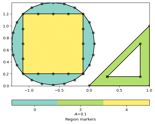
- pygimli.meshtools.createPolygon(verts, isClosed=False, addNodes=0, interpolate='linear', **kwargs)[source]#
Create a polygon from a list of vertices.
All vertices need to be unique and duplicate vertices will be ignored. If you want the polygon be a closed region you can set the ‘isClosed’ flag. Closed region can be attributed by assigning a region marker. The automatic region marker is placed in the center of all vertices.
- Parameters:
verts ([]) –
List of x y pairs [[x0, y0], … ,[xN, yN]]
isClosed (bool [True]) – Add closing edge between last and first node.
addNodes (int [1], iterable) – Constant or (for each) Number of additional nodes to be added, equidistant between sensors.
interpolate (str ['linear']) – Interpolation rule for addNodes. ‘linear’ or ‘spline’. TODO ‘harmfit’
**kwargs –
- markerint [None]
Marker for the resulting triangle cells after mesh generation.
- markerPositionfloats [x, y] [0.0, 0.0]
Position (absolute) of the marker (works for both regions and holes)
- areafloat [0]
Maximum cell size for resulting triangles after mesh generation
- isHolebool [False]
The polygon will become a hole instead of a triangulation
- boundaryMarkerint [1]
Marker for the resulting boundary edges
- leftDirectionbool [True]
Rotational direction
- Returns:
poly – The resulting polygon is a GIMLI::Mesh.
- Return type:
Examples
>>> # no need to import matplotlib, pygimli show does.
>>> import pygimli as pg
>>> import pygimli.meshtools as mt
>>> p1 = mt.createPolygon([[0.0, 0.0], [1.0, 0.0], [1.0, 1.0]],
...                       isClosed=True, marker=3, area=0.1)
>>> p2 = mt.createPolygon([[0.3, 0.15], [0.85, 0.15], [0.85, 0.7]],
...                       isClosed=True, isHole=True)
>>> p3 = mt.createPolygon([[-0.1, 0.2], [-1.1, 0.2], [-1.1, 1.2], [-0.1, 1.2]],
...                       isClosed=True, addNodes=3, marker=2)
>>> p4 = mt.createPolygon([[-0.1, 0.2], [-1.1, 0.2], [-1.1, 1.2], [-0.1, 1.2]],
...                       isClosed=True, addNodes=5, interpolate='spline',
...                       marker=4)
>>> ax, _ = pg.show(mt.mergePLC([p1, p2, p3, p4]), showNodes=True)
>>> pg.wait()
Examples using pygimli.meshtools.createPolygon
- pygimli.meshtools.createRectangle(start=None, end=None, pos=None, size=None, **kwargs)[source]#
Create rectangle polygon.
Create rectangle with start position and a given size. Give either start and end OR pos and size.
- Parameters:
start ([x, y]) – Left upper corner. Default [-0.5, 0.5]
end ([x, y]) – Right lower corner. Default [0.5, -0.5]
pos ([x, y]) – Center position. The rectangle will be moved.
size ([x, y]) – Factors for x and y by which the rectangle, defined by start and width, are scaled.
- Keyword Arguments:
**kwargs –
Additional kwargs
- markerint [1]
Marker for the resulting triangle cells after mesh generation
- markerPositionfloats [x, y] [pos + (end - start) * 0.2]
Absolute position of the marker (works for both regions and holes).
- areafloat [0]
Maximum cell size for resulting triangles after mesh generation
- isHolebool [False]
The polygon will become a hole instead of a triangulation
- boundaryMarkerint [1]
Marker for the resulting boundary edges
- leftDirectionbool [True]
TODO Rotational direction
- pnts: [[x, y],]
Return squared rectangle of origin-aligned boundingbox for pnts.
- minBB: False
Return squared rectangle of non-origin-aligned minimum bounding box for pnts.
- minBBOffset: [1.0, 1.0]
Offset for minimal boundingbox in x and y direction in relative extent .. whatever that means for non-aligned boxes.
- Returns:
poly – The resulting polygon is a GIMLI::Mesh.
- Return type:
Examples
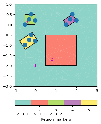
>>> # no need to import matplotlib, pygimli show does.
>>> import pygimli as pg
>>> import pygimli.meshtools as mt
>>> r1 = mt.createRectangle(pos=[1, -1], size=[4.0, 4.0],
...                      marker=1, area=0.1, markerPosition=[0, -2])
>>> r2 = mt.createRectangle(start=[0.5, -0.5], end=[2, -2],
...                      marker=2, area=1.1)
>>> pnts3 = [[-0.5, 0], [0, 0.2], [-0.2, 0.5], [-0.3, 0.25]]
>>> r3 = mt.createRectangle(pnts=pnts3, marker=3, area=0.2)
>>> pnts4 = [[1.5, 0], [2.0, 0.2], [1.8, 0.5], [1.7, 0.25]]
>>> r4 = mt.createRectangle(pnts=pnts4, marker=4, minBB=True)
>>> pnts5 = [[-0.5, -1], [0, -0.8], [-0.2, -0.5], [-0.3, -0.75]]
>>> r5 = mt.createRectangle(pnts=pnts5, marker=5,
...                         minBB=True, minBBOffset=[1.2, 1.2])
>>> ax, _ = pg.show(mt.mergePLC([r1, r2, r3, r4, r5]))
>>> pg.viewer.mpl.drawSensors(ax, pnts3)
>>> pg.viewer.mpl.drawSensors(ax, pnts4)
>>> pg.viewer.mpl.drawSensors(ax, pnts5)
Examples using pygimli.meshtools.createRectangle
- pygimli.meshtools.createSphere(size=None, pos=None, nSegments=20, nRings=10, rot=None, boundaryMarker=0, var='uvsphere', triFaces=True, **kwargs)[source]#
Create sphere PLC as geometrie definition.
Create sphere PLC as geometrie definition. You can either give size and center position.
- Parameters:
size ([x, y, z]) – x, y, and z-size of the cube. Default = [1.0, 1.0, 1.0] in m
pos ([x, y, z]) – The center position, default is at the origin.
nSegments (int[0]) – Discrete number of segments along the horizontal axis
nRings (int[0]) – Discrete number of segments along the vertical axis
rot (pg.Pos [None]) – Rotate on the center.
boundaryMarker (int[0]) – Boundary marker for the resulting faces.
var (str='uvsphere') – Variance of sphere: ‘uvsphere’, ‘qsphere’ or ‘icosphere’.
triFaces (bool [True]) – Output triangular faces instead of quadrilateral faces. Only for qsphere at the moment.
- Keyword Arguments:
kwargs (**) –
- Marker related arguments:
See
pygimli.meshtools.polytools.setPolyRegionMarker
- refine: int [3]
Number of refinements to create a smoother sphere. Default refine=3 for variance=’qsphere’ and refine=2 for ‘icosphere’
- Returns:
poly – The resulting polygon is a GIMLI::Mesh.
- Return type:
Examples
>>> import pygimli as pg
>>> import pygimli.meshtools as mt
>>> sphere = mt.createSphere()
>>> print(sphere)
Mesh: Nodes: 182 Cells: 0 Boundaries: 360
>>> sphere = mt.createSphere()
>>> print(sphere.bb())
[RVector3: (-0.5, -0.5, -0.5), RVector3: (0.5, 0.5, 0.5)]
>>> uvs = mt.createSphere([6, 5, 2], nSegments=25, nRings=15)
>>> pg.show(uvs, showMesh=True, markers=True)
(<pyvista...
>>> uv = pg.meshtools.createSphere(var='uvsphere', pos=[3,0,0])
>>> qs4 = pg.meshtools.createSphere(var='qsphere', pos=[2,0,0],
...                                 refine=3, triFaces=False)
>>> qs3 = pg.meshtools.createSphere(var='qsphere', pos=[1,0,0],
...                                 refine=3, triFaces=True)
>>> ico = pg.meshtools.createSphere(var='icosphere', pos=[0,0,0],
...                                 refine=2)
>>> pg.show([uv, qs4, qs3, ico], showMesh=True,
...         markers=True)
(<pyvista...
- pygimli.meshtools.createSurface(mesh, boundaryMarker=None, verbose=True)[source]#
Convert a 2D mesh into a 3D surface mesh.
- Parameters:
mesh (GIMLI::Mesh) – The 2D input mesh.
boundaryMarker (int[0]) – Boundary marker for the resulting faces. If None the cell markers of the mesh are taken.
- Returns:
The 3D surface mesh.
- Return type:
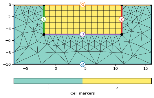
- pygimli.meshtools.createWorld(start, end, marker=1, area=0.0, layers=None, worldMarker=True, **kwargs)[source]#
Create simple rectangular 2D or 3D world.
Create simple rectangular [hexagonal] world with appropriate boundary conditions. Surface boundary is set pg.core.MARKER_BOUND_HOMOGEN_NEUMANN, and inner subsurface is set to pg.core.MARKER_BOUND_MIXED, i.e., -2 OR Numbered: 1, 2, 3, 4, 5, 6 for left, right, bottom, top, front and back, if worldMarker is set to false and no layers are given. With layers, it is numbered in ascending order.
- Parameters:
start ([x, y, [z]]) – Upper/Left/[Front] Corner
end ([x, y, [z]]) – Lower/Right/[Back] Corner
marker (int) – Marker for the resulting triangle cells after mesh generation.
area (float | list) – Maximum cell size for resulting triangles after mesh generation. If area is a float set it global, if area is a list set it per layer.
layers ([float] [None]) – List of depth coordinates for some layers.
worldMarker (bool [True]) – Specify boundary markers: True: [-1, -2] for [surface, subsurface] boundaries False: ascending order [1, 2, 3, 4 ..]
createCube (Forwarded to)
- Returns:
poly – The resulting polygon is a GIMLI::Mesh.
- Return type:
Examples
>>> from pygimli.meshtools import createWorld
>>> from pygimli.viewer.mpl import drawMesh
>>> import matplotlib.pyplot as plt
>>> world = createWorld(start=[-5, 0], end=[5, -5], layers=[-1,-2,-3])
>>>
>>> fig, ax = plt.subplots()
>>> drawMesh(ax, world)
>>> plt.show()
Examples using pygimli.meshtools.createWorld
- pygimli.meshtools.exportFenicsHDF5Mesh(mesh, exportname)[source]#
Exports Gimli mesh in HDF5 format suitable for Fenics.
Equivalent to calling the function
pygimli.meshtools.exportHDF5Mesh(mesh, exportname, group=['mesh', 'domains'], indices='cell_indices', pos='coordinates', cells='topology', marker='values').- Parameters:
mesh (:gimliapi:GIMLI::Mesh`) – Mesh to be saved.
exportname (string) – Name under which the mesh is saved.
- pygimli.meshtools.exportHDF5Mesh(mesh, exportname, group='mesh', indices='cell_indices', pos='coordinates', cells='topology', marker='values')[source]#
Writes given GIMLI::Mesh in a hdf5 format file.
3D tetrahedral meshes only! Boundary markers are ignored.
Keywords are explained in
pygimli.meshtools.readHDFS
- pygimli.meshtools.exportPLC(poly, fname, **kwargs)[source]#
Export a piece-wise linear complex (PLC) to a .poly file (2D or 3D).
Chooses from poly.dimension() and forwards accordingly to poly.exportAsTetgenPolyFile or
pygimli.meshtools.writeTrianglePoly- Parameters:
poly (GIMLI::Mesh) – The polygon to be written.
fname (string) – Filename of the file to write (\*.n, \*.e).
Examples
>>> import pygimli as pg
>>> import tempfile, os
>>> fname = tempfile.mktemp() + '.poly' # Create temporary filename.
>>> world2d = pg.meshtools.createWorld(start=[-10, 0], end=[20, -10])
>>> pg.meshtools.exportPLC(world2d, fname)
>>> read2d = pg.meshtools.readPLC(fname)
>>> print(read2d)
Mesh: Nodes: 4 Cells: 0 Boundaries: 4
>>> world3d = pg.createGrid([0, 1], [0, 1], [-1, 0])
>>> pg.meshtools.exportPLC(world3d, fname)
>>> os.remove(fname)
See also
- pygimli.meshtools.exportSTL(mesh, fileName, binary=False)[source]#
Write STL surface mesh and returns a GIMLI::Mesh.
Export a three dimensional boundary GIMLI::Mesh into a STL surface mesh. Boundaries with different marker will be separated into different STL solids.
- Parameters:
mesh (GIMLI::Mesh) – Mesh to be exported. Only Boundaries of type TriangleFace will be exported.
fileName (str) – name of the .stl file containing the STL surface mesh
binary (bool [False]) – Write STL binary format. TODO
- pygimli.meshtools.extract2dSlice(mesh, origin=None, normal=None, angle=0, dip=0, **kwargs)[source]#
Extract slice from 3D mesh as triangle mesh.
- Parameters:
mesh (pg.Mesh) – Input mesh
origin ([float, float, float]) – origin to be shifted [x, y, z]
normal ([float, float, float] | str) – normal vector for extracting plane, or “x”, “y”, “z” equal to “yz”, “xz”, “yz”, OR
angle (float [0]) – azimuth of plane in the xy plane (0=x, 90=y)
dip (float [0]) – angle to be tilted into the x’z plane (0=vertical)
keywords (Optional)
-----------------
x (float [None]) – axis-parallel flices, determines normal and origin
y (float [None]) – axis-parallel flices, determines normal and origin
z (float [None]) – axis-parallel flices, determines normal and origin
- Return type:
2d triangular pygimli mesh with all data fields
Examples using pygimli.meshtools.extract2dSlice
- pygimli.meshtools.extractUpperSurface2dMesh(mesh, zCut=None)[source]#
Extract 2d mesh from the upper surface of a 3D mesh.
Useful for showing a quick 2D plot of a 3D parameter distribution All cell-based parameters are copied to the new mesh
- Parameters:
mesh (GIMLI::Mesh) – Input mesh (3D)
zCut (float) – z value to distinguish between top and bottom
- Returns:
mesh2d – output 2D mesh consisting of triangles or quadrangles
- Return type:
Examples
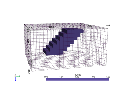
>>> import pygimli as pg
>>> from pygimli.meshtools import extractUpperSurface2dMesh
>>> mesh3d = pg.createGrid(5, 4, 3)
>>> mesh3d["val"] = pg.utils.grange(0, mesh3d.cellCount(), 1)
>>> mesh2d = extractUpperSurface2dMesh(mesh3d)
>>> ax, _ = pg.show(mesh2d, "val")

- pygimli.meshtools.extrude(p2, z=-1.0, boundaryMarker=0, **kwargs)[source]#
Create 3D body by extruding a closed 2D poly into z direction.
- Parameters:
p2 (GIMLI::Mesh) – 2D geometry
z (float [-1.0]) – 2D geometry
- Keyword Arguments:
kwargs (**) – Marker related arguments: See
pygimli.meshtools.polytools.setPolyRegionMarker- Returns:
poly – The resulting polygon is a GIMLI::Mesh.
- Return type:
- pygimli.meshtools.extrudeMesh(mesh, a, **kwargs)[source]#
Extrude mesh to a higher dimension.
Generates a 2D mesh by extruding a 1D mesh along y-coordinate using quads. We assume a 2D mesh here consisting of nodes and edges. The marker of nodes are extruded as edges with the same marker. The marker of the edges are extruded as cells with same marker. Optionally all y-coordinates can be adjusted to become equal at the end
Generates a three-dimensional mesh by extruding a two-dimensional mesh along the z-coordinate transforming triangles into triangular prisms or quads into hexahedrons. 3D cell markers are set from 2D cell marker. The boundary marker for the side boundaries are set from edge markers.
- Parameters:
mesh (GIMLI::Mesh) – Input mesh
a (iterable (float)) – Additional coordinate to extrude into.
- Keyword Arguments:
adjustBottom (bool [False]) – Adjust all nodes such that the bottom of the mesh has a constant depth (only 2D)
- Returns:
mesh – Returning mesh of +1 dimension
- Return type:
Examples
>>> import numpy as np
>>> import pygimli as pg
>>> import pygimli.meshtools as mt
>>> topo = [[x, 1.0 + np.cos(2 * np.pi * 1/30 * x)] for x in range(31)]
>>> m1 = mt.createPolygon(topo)
>>> m1.setBoundaryMarkers(range(m1.boundaryCount()))
>>> m = mt.extrudeMesh(m1, a=-(np.geomspace(1, 5, 8)-1.0))
>>> _ = pg.show(m, m.cellMarkers(), showMesh=True)
>>> m = mt.extrudeMesh(m1, a=-(np.geomspace(1, 5, 8)-1.0),
...                    adjustBottom=True)
>>> _ = pg.show(m, m.cellMarkers(), showMesh=True)


Examples using pygimli.meshtools.extrudeMesh
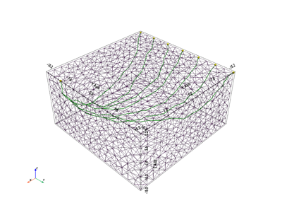
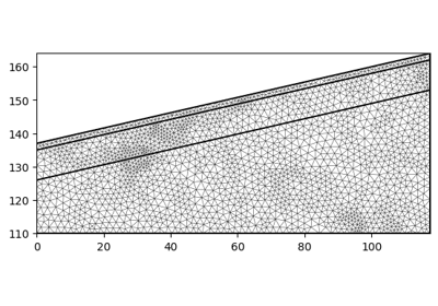
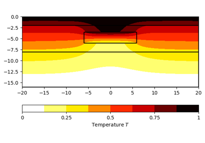
- pygimli.meshtools.fillEmptyToCellArray(mesh, vals, slope=True)[source]#
Prolongate empty cell values to complete cell attributes.
It is possible to have zero values that are filled with appropriate attributes. This function tries to fill empty values successively by prolongation of the non-zeros.
- Parameters:
mesh (GIMLI::Mesh) – For each cell of mesh a value will be returned.
vals (array) – Array of size cellCount().
- Returns:
atts – Array of length mesh.cellCount()
- Return type:
array
Examples
>>> import pygimli as pg
>>> import pygimli.meshtools as mt
>>> import numpy as np
>>> import matplotlib.pyplot as plt
>>>
>>> # Create a mesh with 3 layers and an outer region for extrapolation
>>> layers = mt.createWorld([0,-50],[100,0], layers=[-15,-35])
>>> inner = mt.createMesh(layers, area=3)
>>> mesh = mt.appendTriangleBoundary(inner, xbound=120, ybound=50,
...                                  area=20, marker=0)
>>>
>>> # Create data for the inner region only
>>> layer_vals = [20,30,50]
>>> data = np.array(layer_vals)[inner.cellMarkers() - 1]
>>>
>>> # The following fails since len(data) != mesh.cellCount(), extrapolate
>>> # pg.show(mesh, data)
>>>
>>> # Create data vector, where zeros fill the outer region
>>> data_with_outer = np.array([0] + layer_vals)[mesh.cellMarkers()]
>>>
>>> # Actual extrapolation
>>> extrapolated_data = mt.fillEmptyToCellArray(mesh,
...                                  data_with_outer, slope=False)
>>> extrapolated_data_with_slope = mt.fillEmptyToCellArray(mesh,
...                                 data_with_outer, slope=True)
>>>
>>> # Visualization
>>> fig, (ax1, ax2, ax3) = plt.subplots(1,3, figsize=(10,8), sharey=True)
>>> _ = pg.show(mesh, data_with_outer, ax=ax1, cMin=0)
>>> _ = pg.show(mesh, extrapolated_data, ax=ax2, cMin=0)
>>> _ = pg.show(mesh, extrapolated_data_with_slope, ax=ax3, cMin=0)
>>> _ = ax1.set_title("Original data")
>>> _ = ax2.set_title("Extrapolated with slope=False")
>>> _ = ax3.set_title("Extrapolated with slope=True")
- pygimli.meshtools.fromSubsurface(obj, order='C', verbose=False)[source]#
Convert subsurface object to pygimli mesh.
See more: https://softwareunderground.github.io/subsurface/
Order refers to np.flatten(order) strategy for structured cell data arrangement, e.g., use ‘F’ (Fortran style) for gempy meshes. Default is ‘C’-Style.
Testet objects so far:
TriSurf
UnstructuredData (3D Boundary from TriSurf)
StructuredData (3D cell centered voxel)
- Parameters:
obj (obj) – Subsurface obj, mesh object
order (str ['C']) – Flatten style for structured data attributes. See above.
verbose (boolean [False]) – Be verbose during import.
- Returns:
mesh
- Return type:
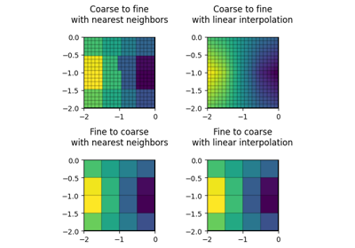
- pygimli.meshtools.interpolate(*args, **kwargs)[source]#
Interpolate different kind of data.
Convenience function for different interpolation schemes:
- 1. Interpolate mesh based data from one mesh to another
syntactic sugar for the core based pg.core.interpolate
- Parameters:
args (GIMLI::Mesh, GIMLI::Mesh, values) –
outData = pg.core.interpolate(outMesh, inMesh, values)
Interpolated values based on inMesh to outMesh.
Values can be of length inMesh.cellCount() interpolated to outMesh.cellCenters(), or inMesh.nodeCount() which are interpolated to outMesh.positions().
- Return type:
Interpolated values.
- 2. Mesh based values to arbitrary points, based on finite elements
syntactic sugar for the core based pg.core.interpolate
- Parameters:
args (GIMLI::Mesh, …) – Arguments forwarded to GIMLI::interpolate()
kwargs –
Arguments forwarded to GIMLI::interpolate()
interpolate(srcMesh, destMesh) All data from inMesh are interpolated to outMesh
- Return type:
Interpolated values
- 3. Interpolate along curve.
Forwarded to
pygimli.meshtools.interpolateAlongCurve
- Parameters:
args (curve, t)
kwargs – Arguments forwarded to
pygimli.meshtools.interpolateAlongCurveperiodic (bool [False]) – Curve is periodic. Useful for closed parametric spline interpolation.
- 4. 1D interpolation
1D point set \(u(x)\) for ascending \(x\). Find interpolation function \(I = u(x)\) and returns \(u_{\text{i}} = I(x_{\text{i}})\) (interpolation methods are [linear via matplotlib, cubic spline via scipy, fit harmonic functions’ via pygimli]) Note, for ‘linear’ and ‘spline’ the interpolate contains all original coordinates while ‘harmonic’ returns an approximate best fit. The amount of harmonic coefficients can be specified by the ‘nc’ keyword.
- Parameters:
args (xi, x, u) –
\(x_{\text{i}}\) - target sample points
\(x\) - function sample points
\(u\) - function values
kwargs –
- methodstring
Specify interpolation method ‘linear, ‘spline’, ‘harmonic’
- ncint
Number of harmonic coefficients for the ‘harmonic’ method.
- periodicbool [False]
Curve is periodic. Useful for closed parametric spline interpolation.
- Returns:
ui – \(u_{\text{i}} = I(x_{\text{i}})\), with \(I = u(x)\)
- Return type:
array of length xi
To use the core functions GIMLI::interpolate() start with a mesh instance as first argument or use the appropriate keyword arguments.
Examples
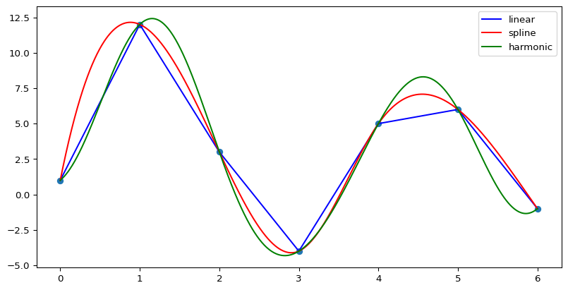
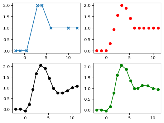
>>> import numpy as np
>>> import pygimli as pg
>>> fig, ax = pg.plt.subplots(1, 1, figsize=(10, 5))
>>> u = np.array([1.0, 12.0, 3.0, -4.0, 5.0, 6.0, -1.0])
>>> xu = np.array(range(len(u)))
>>> xi = np.linspace(xu[0], xu[-1], 1000)
>>> _= ax.plot(xu, u, 'o')
>>> _= ax.plot(xi, pg.interpolate(xi, xu, u, method='linear'),
...         color='blue', label='linear')
>>> _= ax.plot(xi, pg.interpolate(xi, xu, u, method='spline'),
...            color='red', label='spline')
>>> _= ax.plot(xi, pg.interpolate(xi, xu, u, method='harmonic'),
...         color='green', label='harmonic')
>>> _= ax.legend()
>>>
>>> pg.plt.show()
- pygimli.meshtools.interpolateAlongCurve(curve, t, **kwargs)[source]#
Interpolate along curve.
Return curve coordinates for a piecewise linear curve \(C(t) = {x_i,y_i,z_i}\) at positions \(t\). Curve and \(t\) values are expected to be sorted along distance from the origin of the curve.
- Parameters:
curve ([[x,z]] | [[x,y,z]] | [GIMLI::Pos,]) – Discrete curve for 2D \(x,z\) curve=[[x,z]], 3D \(x,y,z\)
t (1D iterable) – Query positions along the curve in absolute distance
kwargs –
If kwargs are given, an additional curve smoothing is applied using
pygimli.meshtools.interpolate. The kwargs will be delegated.- periodicbool [False]
Curve is periodic. Usefull for closed parametric spline interpolation.
- Returns:
p – Curve positions at query points \(t\). Dimension of p match the size of curve the coordinates.
- Return type:
np.array
Examples
>>> import numpy as np
>>> import pygimli as pg
>>> import pygimli.meshtools as mt
>>> fig, axs = pg.plt.subplots(2,2)
>>> topo = np.array([[-2., 0.], [-1., 0.], [0.5, 0.], [3., 2.], [4., 2.], [6., 1.], [10., 1.], [12., 1.]])
>>> t = np.arange(15.0)
>>> p = mt.interpolateAlongCurve(topo, t)
>>> _= axs[0,0].plot(topo[:,0], topo[:,1], '-x', mew=2)
>>> _= axs[0,1].plot(p[:,0], p[:,1], 'o', color='red')
>>>
>>> p = mt.interpolateAlongCurve(topo, t, method='spline')
>>> _= axs[1,0].plot(p[:,0], p[:,1], '-o', color='black')
>>>
>>> p = mt.interpolateAlongCurve(topo, t, method='harmonic', nc=3)
>>> _= axs[1,1].plot(p[:,0], p[:,1], '-o', color='green')
>>>
>>> pg.plt.show()
- pygimli.meshtools.merge(*args, **kwargs)[source]#
Little syntactic sugar to merge.
All args are forwarded to mergeMeshes if isGeometry is not set. Otherwise it considers the mesh as PLC to merge.
- Parameters:
to (List of meshes or comma separated list of meshes that will be forwarded)
meshPLC. (mergeMeshes or)
- pygimli.meshtools.merge2Meshes(m1, m2)[source]#
Merge two meshes into one new mesh and return the combined mesh.
Merge two meshes into a new mesh and return the combined mesh. Note that there is a duplicate check for all nodes which should reuse existing node but NO cells or boundaries.
- Parameters:
m1 (GIMLI::Mesh) – First mesh.
m2 (GIMLI::Mesh) – Second mesh.
- Returns:
mesh – Resulting mesh.
- Return type:
- pygimli.meshtools.mergeMeshes(meshList, verbose=False)[source]#
Merge several meshes into one new mesh and return the new mesh.
Merge several meshes into one new mesh and return the new mesh.
- Parameters:
meshList ([GIMLI::Mesh, …] | [str, …]) – List of at least two meshes (or filenames to meshes) to be merged.
verbose (bool) – Give some output
See also
Examples using pygimli.meshtools.mergeMeshes
- pygimli.meshtools.mergePLC(plcs, tol=0.001)[source]#
Merge multiply polygons.
Merge multiply polygons into a single polygon. Common nodes and common edges will be checked and removed. When a node touches an edge, the edge will be split.
3D only OOC with polytools.
- Parameters:
plcs ([GIMLI::Mesh,]) – List of PLC that want to be merged into one new PLC
tol (double) – Tolerance to check for duplicated nodes. [1e-3]
- Returns:
plc – The resulting polygon is a GIMLI::Mesh.
- Return type:
Examples
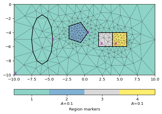
>>> import pygimli as pg
>>> import pygimli.meshtools as mt
>>> from pygimli.viewer.mpl import drawMesh
>>> world = mt.createWorld(start=[-10, 0], end=[10, -10], marker=1)
>>> c1 = mt.createCircle([-1, -4], radius=1.5, area=0.1,
...                       marker=2, nSegments=5)
>>> c2 = mt.createCircle([-6, -5], radius=[1.5, 3.5], isHole=1)
>>> r1 = mt.createRectangle(pos=[3, -5], size=[2, 2], marker=3)
>>> r2 = mt.createRectangle(start=[4, -4], end=[6, -6],
...                          marker=4, area=0.1)
>>> plc = mt.mergePLC([world, c1, c2, r1, r2])
>>> fig, ax = pg.plt.subplots()
>>> drawMesh(ax, plc)
>>> drawMesh(ax, mt.createMesh(plc))
>>> pg.wait()
Examples using pygimli.meshtools.mergePLC
- pygimli.meshtools.mergePLC3D(plcs, tol=0.001)[source]#
Merge a list of 3D PLC into one.
Experimental replacement for polyMerge. Don’t expect too much.
- Works if:
all plcs are free and does not have any contact to each other
contact of two facets if the second is completely within the first
- pygimli.meshtools.nodeDataToBoundaryData(mesh, data)[source]#
Convert node data to boundary data.
Assuming [NodeCount, dim] data DOCUMENT_ME
- pygimli.meshtools.nodeDataToCellData(mesh, data)[source]#
Convert node data to cell data.
Convert node data to cell data via interpolation to cell centers.
- Parameters:
mesh (GIMLI::Mesh) – 2D or 3D GIMLi mesh
data (iterable [float]) – Data of len mesh.nodeCount(). TODO complex, R3Vector, ndarray
Examples using pygimli.meshtools.nodeDataToCellData
- pygimli.meshtools.quality(mesh, measure='eta')[source]#
Return the quality of a given triangular mesh.
- Parameters:
mesh (mesh object) – Mesh for which the quality is calculated.
measure (quality measure, str) – Can be either “eta”, “nsr”, or “minimumAngle”.
Examples
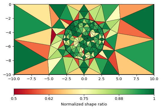
>>> # no need to import matplotlib
>>> import pygimli as pg
>>> from pygimli.meshtools import polytools as plc
>>> from pygimli.meshtools import quality
>>> # Create Mesh
>>> world = plc.createWorld(start=[-10, 0], end=[10, -10],
...                         marker=1, worldMarker=False)
>>> c1 = plc.createCircle(pos=[0.0, -5.0], radius=3.0, area=.3)
>>> mesh = pg.meshtools.createMesh([world, c1], quality=21.3)
>>> # Compute and show quality
>>> q = quality(mesh, measure="nsr")
>>> ax, _ = pg.show(mesh, q, cMap="RdYlGn", showMesh=True, cMin=0.5,
...                 cMax=1.0, label="Normalized shape ratio")

See also
eta,nsr,minimumAngle
Examples using pygimli.meshtools.quality
- pygimli.meshtools.readFenicsHDF5Mesh(fileName, verbose=True, **kwargs)[source]#
Reads FEniCS mesh from file format .h5 and returns a GIMLI::Mesh.
- pygimli.meshtools.readGmsh(fName, verbose=False, precision=None)[source]#
Read Gmsh ASCII file and return instance of GIMLI::Mesh class.
- Parameters:
fName (string) – Filename of the file to read (\*.msh). The file must conform to the MSH ASCII file version 2 format
verbose (boolean, optional) – Be verbose during import. Default: False
precision (None|int, optional) – If not None, then round off node coordinates to the provided number of digits using numpy.round. This is useful in case that nodes are accessed using their coordinates, in which case numerical discrepancies can occur.
Notes
Physical groups specified in Gmsh are interpreted as follows:
Points with the physical number 99 are interpreted as sensors. Note that physical point groups are ordered with respect to the node tag. E.g. “Physical Point (99) = {50, 34};” and “Physical Point (99) = {34, 50};” will yield the same mesh. This must be taken into account when defining measurement configurations using electrodes defined in GMSH using marker 99.
ERT only: Points with markers 999 and 1000 are used to mark calibration and reference nodes.
- Physical Lines and Surfaces define boundaries in 2D and 3D, respectively.
Physical Number 1: Homogeneous Neumann condition
Physical Number 2: Mixed boundary condition
Physical Number 3: Homogeneous Dirichlet condition
Physical Number 4: Dirichlet condition
- Physical Surfaces and Volumes define regions in 2D and 3D, respectively.
Physical Number 1: No inversion region
Physical Number >= 2: Inversion region
Examples
>>> import tempfile, os
>>> from pygimli.meshtools import readGmsh
>>> gmsh = '''
... $MeshFormat
... 2.2 0 8
... $EndMeshFormat
... $Nodes
... 3
... 1 0 0 0
... 2 0 1 0
... 3 1 1 0
... $EndNodes
... $Elements
... 7
... 1 15 2 0 1 1
... 2 15 2 0 2 2
... 3 15 2 0 3 3
... 4 1 2 0 1 2 3
... 5 1 2 0 2 3 1
... 6 1 2 0 3 1 2
... 7 2 2 0 5 1 2 3
... $EndElements
... '''
>>> fName = tempfile.mktemp()
>>> with open(fName, "w") as f:
...     f.writelines(gmsh)
>>> mesh = readGmsh(fName)
>>> print(mesh)
Mesh: Nodes: 3 Cells: 1 Boundaries: 3
>>> os.remove(fName)
Examples using pygimli.meshtools.readGmsh
- pygimli.meshtools.readHDF5Mesh(fileName, group='mesh', indices='cell_indices', pos='coordinates', cells='topology', marker='values', marker_default=0, dimension=3, verbose=True, useFenicsIndices=False)[source]#
Function for loading a mesh from HDF5 file format.
Returns an instance of GIMLI::Mesh class. Default values for keywords are suited for FEniCS syntax .h5 meshes.
Requirements: h5py module
- Parameters:
fileName (string) – Name of the mesh to be transformed into pyGIMLi format.
group (string ['domains']) – hdf group that contains the mesh information (see other keyword arguments). Default is ‘domains’ for FEniCS compatibility.
indices (string ['cell_indices']) – Key for the part of the hdf file containing the indices of the cells.
pos (string ['coordinates']) – Key for the part of the hdf file containing the nodepositions.
cells (string ['topology']) – Key for the part of the hdf file containing the array which defies the cells. Usually of shape (cellCount, 3) for 2D meshes or (cellCount, 4) for 3D tetrahedra meshes. For each cell the indices of the corresponding node indices is given.
marker (string ['values']) – If marker is part of the hdf data container, the corresponding array is used as identifier for the cell markers. If not found, the cell markers will be set to marker_default.
marker_default (int or array [0]) – Default marker if no markers are found in the hdf file. If array, size has to match the cellCount of the mesh.
dimension (int [3]) – Dimension of the input/output mesh, no own check for dimensions yet. Fixed on 3 for now.
- Returns:
- Return type:
mesh
- pygimli.meshtools.readHydrus2dMesh(fileName='MESHTRIA.TXT')[source]#
Import mesh from Hydrus2D.
- Parameters:
fName (str, optional) – Filename of Hydrus output file.
See also
readHydrus3dMeshSimilar routine for three-dimensional meshes.
References
- pygimli.meshtools.readHydrus3dMesh(fileName='MESHTRIA.TXT')[source]#
Import mesh from Hydrus3D.
- Parameters:
fName (str, optional) – Filename of Hydrus output file.
See also
readHydrus2dMeshSimilar routine for two-dimensional meshes.
References
- pygimli.meshtools.readMeshIO(fileName, verbose=False)[source]#
Generic mesh read using meshio. (nschloe/meshio)
- pygimli.meshtools.readPLC(filename: str, comment: str = '#')[source]#
Read in a piece-wise linear complex object (PLC) from .poly file.
Read 2D Triangle or 3D Tetgen PLC files.
- Parameters:
filename (string) – Filename *.poly
comment (string) – String containing all characters that define a comment line. Identified lines will be ignored during import.
- Returns:
- Return type:
poly
See also
- pygimli.meshtools.readSTL(fileName, binary=False)[source]#
Read STL surface mesh and returns a GIMLI::Mesh.
Read STL surface mesh and returns a GIMLI::Mesh of triangle boundary faces. Multiple solids are supported with increasing boundary marker.
TODO: ASCII=False, read binary STL
- Parameters:
fileName (str) – name of the .stl file containing the STL surface mesh
binary (bool [False]) – STL Binary format
- pygimli.meshtools.readTetgen(fName, comment='#', verbose=False, defaultCellMarker=0, loadFaces=True, quadratic=False)[source]#
Read and convert a mesh from the basic Tetgen output.
Read Tetgen [Si, 2004] ASCII files and return instance of GIMLI::Mesh class. See: http://tetgen.org/
- Parameters:
fName (str) – Base name of the tetgen output, without ending. All additional files (.node, .ele and .face) need to have the same basename.
comment (str ('#')) – String consisting of all symbols indicating a comment in the input files. Standard for tetgen files is the ‘#’.
verbose (boolean (True)) – Enables console output during the import process.
defaultCellMarker (int (0)) – Tetgen files can contain cell markers, but do not have to. If no markers are found, the given integer is used.
loadFaces – Optional decision whether the faces of Tetgen output (.face) are loaded or not. Note that without the -f in during the tetgen call, the faces in the .face file will only contain the faces of the original input poly file and not all faces. If only a part of the faces are imported, a createNeighborInfos call of the mesh will fail.
quadratic (boolean (False)) – Returns a P2 (quadratic) refined mesh when True (to be removed, as soon as direct import of quadratic meshes is possible).
- Returns:
mesh
- Return type:
- pygimli.meshtools.readTriangle(fName, verbose=False)[source]#
Read Triangle [Shewchuk, 1996] mesh.
Read Triangle [Shewchuk, 1996] ASCII mesh files and return an instance of GIMLI::Mesh class. See: ://www.cs.cmu.edu/~quake/triangle.html
- Parameters:
fName (string) – Filename of the file to read (\*.n, \*.e)
verbose (boolean, optional) – Be verbose during import.
- pygimli.meshtools.refineHex2Tet(mesh, style=1)[source]#
Refine mesh of hexahedra into a mesh of tetrahedra.
- Parameters:
mesh (GIMLI::Mesh) – Mesh containing hexrahedron cells, e.g., from a grid.
style (int [1]) –
- 1 bisect each hexahedron int 6 tetrahedrons
(less numerical quality but no problems due to diagonal face split)
- 2 bisect each hexahedron int 5 tetrahedrons
(leads to inconsistent meshes. Neighboring cell have different face split diagonal. Might be fixable by rotating the split order depending on coordinates for every 2nd split)
- Returns:
ret – Mesh containing tetrahedrons cells.
- Return type:
Examples
>>> import pygimli as pg
>>> import pygimli.meshtools as mt
>>> hex = pg.createGrid(2, 2, 2)
>>> print(hex)
Mesh: Nodes: 8 Cells: 1 Boundaries: 6
>>> tet = mt.refineHex2Tet(hex, style=1)
>>> print(tet)
Mesh: Nodes: 8 Cells: 6 Boundaries: 12
>>> tet = mt.refineHex2Tet(hex, style=2)
>>> print(tet)
Mesh: Nodes: 8 Cells: 5 Boundaries: 12
- pygimli.meshtools.refineQuad2Tri(mesh, style=1)[source]#
Refine mesh of quadrangles into a mesh of triangle cells.
TODO mixed meshes
- Parameters:
mesh (GIMLI::Mesh) – Mesh containing quadrangle cells.
style (int [1]) –
1 bisect each quadrangle into 2 triangles
2 cross-sect each quadrangle into 4 triangles
- Returns:
ret – Mesh containing triangle cells.
- Return type:
Examples
>>> import pygimli as pg
>>> import pygimli.meshtools as mt
>>> quads = pg.createGrid(range(10), range(10))
>>> ax, _ = pg.show(quads)
>>> ax, _ = pg.show(mt.refineQuad2Tri(quads, style=1))
>>> ax, _ = pg.show(mt.refineQuad2Tri(quads, style=2))
>>> pg.wait()


- pygimli.meshtools.syscallTetgen(filename, quality=1.2, area=0, preserveBoundary=False, verbose=False, tetgen='tetgen')[source]#
Create a mesh from a PLC by system-calling Tetgen.
Create a Tetgen [Si, 2004] mesh from a PLC.
- Parameters:
filename (str)
quality (float [1.2]) – Refines mesh (to improve mesh quality). [1.1 … ]
area (float [0.0]) – Maximum cell size (m³)
preserveBoundary (bool [False]) – Preserve PLC boundary mesh
verbose (bool [False]) – be verbose
tetgen (str | path ['tetgen']) – Binary for tetgen. Given as complete path or simple the binary name if its known in the system path.
- Returns:
mesh
- Return type:
- pygimli.meshtools.tapeMeasureToCoordinates(tape, pos)[source]#
Interpolate 2D tape measured topography to 2D Cartesian coordinates.
Tape and pos value are expected to be sorted along distance to the origin.
DEPRECATED will be removed, use
pygimli.meshtools.interpolateAlongCurveinsteadTODO optional smooth curve with harmfit TODO parametric TODO parametric + Topo: 3d
- Parameters:
tape ([[x,z]] | [RVector3] | R3Vector) – List of tape measured topography points with measured distance (x) from origin and height (z)
pos (iterable) – Array of query positions along the tape measured profile t[0 ..
- Returns:
res – Same as pos but with interpolated height values. The Distance between pos points and res (along curve) points remains.
- Return type:
ndarray(N, 2)
- pygimli.meshtools.toSubsurface(mesh, verbose=False)[source]#
Create a subsurface object from pygimli mesh.
Testet objects so far:
Creates Subsurface.TriSurf from 3D triangle boundaries
- Parameters:
mesh (GIMLI::Mesh)
verbose (boolean [False]) – Be verbose during import.
- Return type:
Subsurface object depending on input mesh