Complex-valued electrical modelling

In this example, an electrical complex-valued forward modelling is conducted. The use of complex resistivities implies an out-of-phase polarization response of the subsurface, commonly being measured in the frequency domain as complex resistivity (CR), or, if multiple frequencies are measured, also referred to as spectral induced polarization (SIP). Please note that the time-domain induced polarization (TDIP) is a compound signature over a wide range of frequencies.

It is common to parameterize the complex resistivities using magnitude (in \(\Omega`m) and phase :math:\)phi` (in mrad), although the pyGIMLi forward operator takes real and imaginary parts.

import numpy as np
import matplotlib.pylab as plt

import pygimli as pg
import pygimli.meshtools as mt
from pygimli.physics import ert

Create a measurement scheme for 51 electrodes with a spacing of 1m

scheme = ert.createData(
    elecs=np.linspace(start=0, stop=50, num=51),
    schemeName='dd'
)

Mesh generation

world = mt.createWorld(
    start=[-55, 0], end=[105, -80], worldMarker=True)

polarizable_anomaly = mt.createCircle(
    pos=[40, -7], radius=5, marker=2
)

plc = world + polarizable_anomaly

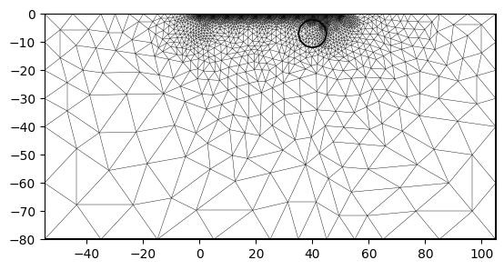
# local refinement of mesh near electrodes
for s in scheme.sensors():
    plc.createNode(s + [0.0, -0.2])

mesh_coarse = mt.createMesh(plc, quality=33)
# additional refinements
mesh = mesh_coarse.createH2()

# Create a P2-optimized mesh (quadratic shape functions)
mesh = mesh.createP2()

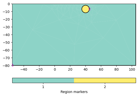
pg.show(plc, marker=True)
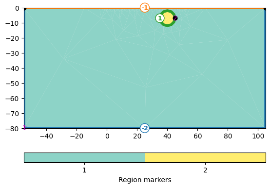
pg.show(plc, markers=True)
pg.show(mesh)

• 
• 
• 

(<Axes: >, None)

Prepare the model parameterization We have two markers here: 1: background 2: circle anomaly Parameters must be specified as a complex number, here converted by the utility function pygimli.utils.complex.toComplex().

rhomap = [
    [1, pg.utils.complex.toComplex(100, 0 / 1000)],
    # Magnitude: 100 ohm m, Phase: -50 mrad
    [2, pg.utils.complex.toComplex(100, -50 / 1000)],
]

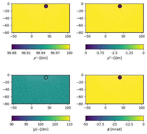
# For visualization, map the rhomap into the actual mesh, resulting in a rho
# vector with a complex resistivity associated with each mesh cell.
rho = pg.solver.parseArgToArray(rhomap, mesh.cellCount(), mesh)
fig, axes = plt.subplots(2, 2, figsize=(16 / 2.54, 16 / 2.54))
pg.show(mesh, data=np.real(rho), ax=axes[0, 0], label=r"$\rho'$~[$\Omega$m]")
pg.show(mesh, data=np.imag(rho), ax=axes[0, 1], label=r"$\rho''$~[$\Omega$m]")
pg.show(mesh, data=np.abs(rho), ax=axes[1, 0], label=r"$|\rho$|~[$\Omega$m]")
pg.show(
    mesh, data=np.arctan2(np.imag(rho), np.real(rho))*1000,
    ax=axes[1, 1], label=r"$\phi$ [mrad]"
)
fig.tight_layout()
fig.show()

Do the actual forward modelling

data = ert.simulate(
    mesh,
    res=rhomap,
    scheme=scheme,
    # noiseAbs=0.0,
    # noiseLevel=0.0,
)

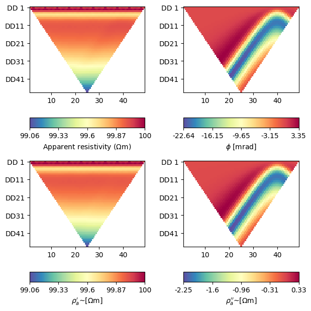
Visualize the modeled data Convert magnitude and phase into a complex apparent resistivity

rho_a_complex = data['rhoa'].array() * np.exp(1j * data['phia'].array())

# Please note the apparent negative (resistivity) phases!
fig, axes = plt.subplots(2, 2, figsize=(16 / 2.54, 16 / 2.54))
ert.showERTData(data, vals=data['rhoa'], ax=axes[0, 0])
# phia is stored in radians, but usually plotted in milliradians
ert.showERTData(
    data, vals=data['phia'] * 1000, label=r'$\phi$ [mrad]', ax=axes[0, 1])

ert.showERTData(
    data, vals=np.real(rho_a_complex), ax=axes[1, 0],
    label=r"$\rho_a'$~[$\Omega$m]"
)
ert.showERTData(
    data, vals=np.imag(rho_a_complex), ax=axes[1, 1],
    label=r"$\rho_a''$~[$\Omega$m]"
)
fig.tight_layout()
fig.show()