pygimli.solver#
General physics independent solver interface.
Overview#
Functions
|
|
|
This should be moved directly into the core |
|
Shortcut to apply all boundary conditions. |
|
Apply Dirichlet boundary condition. |
|
Assemble the load vector. |
|
Apply Neumann condition to the system matrix S. |
|
Apply Robin boundary condition. |
|
Find all boundaries matching a dictionary key. |
|
Get a value for each cell. |
|
Check Courant-Friedrichs-Lewy condition. |
|
|
|
Generic Crank Nicolson solver for time dependend problems. |
|
Create anisotropy matrix with desired properties. |
|
Create constitutive matrix for 2 or 3D isotropic media. |
|
Create a right hand side vector for vector valued solutions. |
|
Create right hand side vector based on the given mesh and load values (scalar solution) or force vectors (vector value solution). |
|
Create the mass matrix. |
|
Create the Stiffness matrix. |
|
Deep copy operation on arbitrary Python objects. |
|
Return the discrete interpolated divergence field. |
|
Divergence for callable function func((x,y,z)). |
|
Generate a value for the given Boundary. |
|
Get map of index: dirichlet value |
|
Return the discrete interpolated gradient \(\mathbf{v}\) for a given scalar field \(\mathbf{u}\). |
|
Greens function for diffusion operator. |
|
Create identity matrix. |
|
Return integral over nodal solution \(u\). |
|
Direct linear solution after \(\textbf{x}\) using core LinSolver. |
|
Create (H1) norm for the finite element space. |
|
Create Lebesgue (L2) norm for finite element space. |
|
Parse boundary related pair argument to create a list of [ GIMLI::Boundary, value|callable ]. |
|
Parse array related arguments to create a valid value array. |
|
Parse boundary related arguments to create a valid boundary value list: [ GIMLI::Boundary, value|callable ] |
|
|
|
Parse a value map to cell attributes. |
|
Parse dictionary key of type str to marker list. |
|
Show the content of a sparse matrix. |
|
Solve partial differential equation. |
|
Solve partial differential equation with Finite Elements. |
|
Solve partial differential equation with Finite Volumes. |
|
Create tri-diagonal Toeplitz matrix. |
Classes
|
Proxy class for the solution of linear systems of equations. |
|
TODO DOCUMENT ME |
Functions#
- pygimli.solver.anisotropyMatrix(*args, **kwargs)#
- pygimli.solver.applyDirichlet(mat, rhs, uDirIndex, uDirichlet)[source]#
This should be moved directly into the core
- pygimli.solver.assembleBC(bc, mesh, mat, rhs, time=None, userData={}, dofOffset=0, nCoeff=1)[source]#
Shortcut to apply all boundary conditions.
Shortcut to apply all boundary conditions will only forward to appropriate assemble functions.
- Returns:
map{id (uDirichlet}: Map of index to Dirichlet value.)
None
- pygimli.solver.assembleDirichletBC(mat, boundaryPairs, rhs=None, time=0.0, userData={}, nodePairs=None, dofOffset=0, nCoeff=1, dofPerCoeff=None)[source]#
Apply Dirichlet boundary condition.
- Parameters:
rhs (
Vector) – Right hand side vector of the system equation will bet set to \(u_{\text{D}}\)
Examples using pygimli.solver.assembleDirichletBC
- pygimli.solver.assembleLoadVector(mesh, f, userData={})[source]#
Assemble the load vector. See createLoadVector.
- pygimli.solver.assembleNeumannBC(rhs, boundaryPairs, nDim=1, time=0.0, userData={}, dofOffset=0, nCoeff=1, dofPerCoeff=None)[source]#
Apply Neumann condition to the system matrix S.
Apply Neumann condition to the system matrix S. The right hand side values for g can be given for each boundary element individually by setting proper boundary pair arguments.
\[\frac{\partial u(\textbf{r}, t)}{\partial\textbf{n}} = \textbf{n}\nabla u(\textbf{r}, t) = g \quad\text{for}\quad\textbf{r}\quad\text{on}\quad\delta\Omega=\Gamma_{\text{Neumann}}\]- Parameters:
rhs (
Vector) – Right hand side vector of length node count.boundaryPair (list()) –
List of pairs [ GIMLI::Boundary, g ]. The value \(g\) will assigned to the nodes of the boundaries. Later assignment overwrites prior.
\(g\) need to be a scalar value (float or int) or a value generator function that will be executed at run time.
See
pygimli.solver.solver.parseArgToBoundariesand Modelling with Boundary Conditions for example syntax,nDim (int [1]) – Number of dimensions for vector valued problems. The rhs array need to have the correct size, i.e., number of Nodes * mesh.dimension()
time (float) – Will be forwarded to value generator.
userData (class) – Will be forwarded to value generator.
dofOffset (int[0]) – Offset for matrix index.
- pygimli.solver.assembleRobinBC(mat, boundaryPairs, rhs=None, time=0.0, userData={}, dofOffset=0, nCoeff=1, dofPerCoeff=None)[source]#
Apply Robin boundary condition.
Apply Robin boundary condition to the system matrix and the rhs vector:
\[\begin{split}\frac{\partial u(\textbf{r}, t)}{\partial\textbf{n}} & = \alpha(u_0-u) \quad\text{or} \\ \beta\frac{\partial u(\textbf{r}, t)}{\partial\textbf{n}} + \alpha u & = \gamma \\ & \quad\text{for}\quad\textbf{r}\quad\text{on}\quad\delta\Omega= \Gamma_{\text{Robin}}\\\end{split}\]- Parameters:
mat (GIMLI::SparseMatrix) – System matrix of the system equation.
boundaryPair (list) –
- List of pairs [GIMLI::Boundary, \(a, u_0\) |
\(\alpha, \beta, \gamma\)].
The values will assigned to the nodes of the boundaries. Later assignment overwrites prior.
Values can be a single value for \(\alpha\) or \(a\), two values will be interpreted as \(a, u_0\), and three values will be \(\alpha, \beta, \gamma\). Also generator (callable) is possible which will be executed at runtime See
pygimli.solver.solver.parseArgToBoundariesModelling with Boundary Conditions or testing/test_FEM.py for example syntax.time (float) – Will be forwarded to value generator.
userData (dict) – Will be forwarded to value generator.
dofOffset (int[0]) – Offset for matrix index.
- pygimli.solver.boundaryIdsFromDictKey(mesh, key, outside=True)[source]#
Find all boundaries matching a dictionary key.
- Variables:
mesh (GIMLI::Mesh) –
key (str|int) – Representation for boundary marker. Will be parsed by
pygimli.solver.solver.parseMarkersDictKeyoutside (bool [True]) – Only select outside boundaries.
- Returns:
dict
- Return type:
{marker, [boundary.id()]}
- pygimli.solver.cellValues(mesh, arg, **kwargs)[source]#
Get a value for each cell.
Returns a array or vector of length mesh.cellCount() based on arg. The preferable arg is a dictionary for the cell marker and the appropriate cell value. The designated value can be calculated using a callable(cell, **kwargs), which is called on demand.
- Variables:
mesh (GIMLI::Mesh) – Used if arg is callable
arg (float | int | complex | ndarray | iterable | callable | dict) –
Argument to be parsed as cell data. If arg is a dictionary, its key will be interpreted as cell marker:
Dictionary is key: value. Value can be float, int, complex or ndarray. The last for anistropic or elastic tensors.
Key can be integer for cell marker or str, which will be interpreted as splice or list. See examples or py:mod:pygimli.solver.parseMarkersDictKey.
Iterable of length mesh.nodeCount() to be interpolated to cell centers.
userData (class) – Used if arg is callable
- Returns:
ret – Array of desired length filled with the appropriate values.
- Return type:
GIMLI::RVector | ndarray(mesh.cellCount(), xx )
Examples
>>> import pygimli as pg
>>> mesh = pg.createGrid(x=range(5))
>>> mesh.setCellMarkers([1, 1, 2, 2])
>>> print(mesh.cellCount())
4
>>> print(pg.solver.cellValues(mesh, [1, 2, 3, 4]))
[1, 2, 3, 4]
>>> print(pg.solver.cellValues(mesh, {1:1.0, 2:10}))
[1.0, 1.0, 10, 10]
>>> print(pg.solver.cellValues(mesh, {':':2.0}))
[2.0, 2.0, 2.0, 2.0]
>>> print(pg.solver.cellValues(mesh, {'0:2':3.0}))
[3.0, 3.0, None, None]
>>> print(pg.solver.cellValues(mesh, np.ones(mesh.nodeCount())))
4 [1.0, 1.0, 1.0, 1.0]
>>> print(np.array(pg.solver.cellValues(mesh, {'1:3' : np.diag([1.0, 2.0])})))
[[[1. 0.]
  [0. 2.]]

 [[1. 0.]
  [0. 2.]]

 [[1. 0.]
  [0. 2.]]

 [[1. 0.]
  [0. 2.]]]
>>> print(np.array(pg.solver.cellValues(mesh, {':' : pg.core.CMatrix(2, 2)})))
[[[0.+0.j 0.+0.j]
  [0.+0.j 0.+0.j]]

 [[0.+0.j 0.+0.j]
  [0.+0.j 0.+0.j]]

 [[0.+0.j 0.+0.j]
  [0.+0.j 0.+0.j]]

 [[0.+0.j 0.+0.j]
  [0.+0.j 0.+0.j]]]
>>> print(pg.solver.cellValues(mesh, {'1,2':1 + 1j*2.0}))
[(1+2j), (1+2j), (1+2j), (1+2j)]
>>> def cellVal(c, b=1):
...     return c.center()[0]*b
>>> t = pg.solver.cellValues(mesh, {':' : cellVal})
>>> print([t[c.id()](c) for c in mesh.cells()])
[0.5, 1.5, 2.5, 3.5]
- pygimli.solver.checkCFL(times, mesh, vMax, verbose=False)[source]#
Check Courant-Friedrichs-Lewy condition.
For advection and flow problems. CFL Number should be lower then 1 to ensure stability.
- pygimli.solver.constitutiveMatrix(*args, **kwargs)#
- pygimli.solver.crankNicolson(times, S, I, f=None, u0=None, theta=1.0, dirichlet=None, solver=None, progress=None)[source]#
Generic Crank Nicolson solver for time dependend problems.
- Limitations so far:
S = Needs to be constant over time (i.e. no change in coefficients) f = constant over time (would need assembling in every step)
- Parameters:
times (iterable(float)) – Timeteps to solve for. Give at least 2.
S (Matrix) – Systemmatrix holds your discrete equations and boundary conditions
I (Matrix) – Identity matrix (FD, FV) or Masselementmatrix (FE) to handle solution vector
u0 (iterable [None]) – Starting condition. zero if not given
f (iterable (float) [None]) – External forces. Note f might also contain compensation values due to algebraic Dirichlet correction of S
theta (float [1.0]) –
0: Backward difference scheme (implicit)
1: Forward difference scheme (explicit)
strong time steps dependency .. will be unstable for to small values * 0.5: probably best tradeoff but can also be unstable
dirichlet (dirichlet generator) – Genertor object to applay dirichlet boundary conditions
solver (LinSolver [None]) – Provide a pre configured solver if you want some special.
progress (Progress [None]) – Provide progress object if you want to see some.
- Returns:
Solution for each time steps
- Return type:
np.ndarray
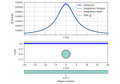
- pygimli.solver.createAnisotropyMatrix(lon, trans, theta)[source]#
Create anisotropy matrix with desired properties.
Anistropy tensor from longitudinal value lon, transverse value trans and the angle theta of the symmetry axis relative to the vertical after cite:WieseGreZho2015 https://www.researchgate.net/publication/249866312_Explicit_expressions_for_the_Frechet_derivatives_in_3D_anisotropic_resistivity_inversion
Examples using pygimli.solver.createAnisotropyMatrix
- pygimli.solver.createConstitutiveMatrix(lam=None, mu=None, E=None, nu=None, dim=2, voigtNotation=False)[source]#
Create constitutive matrix for 2 or 3D isotropic media.
Either give lam and mu or E and nu.
- Parameters:
- Returns:
C – Either 3x3 or 6x6 matrix depending on the dimension
- Return type:
mat
- pygimli.solver.createForceVector(mesh, f, userData={})[source]#
Create a right hand side vector for vector valued solutions.
- Parameters:
f ([ convertable ]) – List of rhs side options. Must be convertable to createLoadVector. See
createLoadVectorrhs (np.array()) – Squeezed vector of length mesh.nodeCount() * mesh.dimensions()
- pygimli.solver.createLoadVector(mesh, f=1.0, userData={})[source]#
Create right hand side vector based on the given mesh and load values (scalar solution) or force vectors (vector value solution).
Create right hand side based on the given mesh and load or force values.
- Parameters:
f (float[1.0], array, callable(cell, [userData]), [f_x, f_y, f_z]) –
- float will be assumed as constant for all cells
like rhs = rhs(np.ones(mesh.cellCount() * f),
- array of length mesh.cellCount() will be processed as load value for
each cell: rhs = rhs(f),
- array of length mesh.nodeCount() is assumed to be already processed
correct: rhs = f
- callable is evaluated on once for each cell and need to return a load
value for each cell and can have optional a userData dictionary: f_cell = f(cell, [userData={}]) rhs = rhs(f(c, userData) for c in mesh.cells())
- list with length of mesh.dimension() of float or array entries will
create a squeezed rhs for vector valued problems rhs = squeeze([rhs(f[0]), rhs(f[1]), rhs(f[2])])
- Returns:
rhs – Right-hand side load vector for scalar values or squeezed vector values
- Return type:
pg.Vector(mesh.nodeCount())
Examples using pygimli.solver.createLoadVector
- pygimli.solver.createMassMatrix(mesh, b=None)[source]#
Create the mass matrix.
Calculates the Mass matrix (Finite element identity matrix) the given mesh.
- ..math::
…
- Parameters:
mesh (GIMLI::Mesh) – Arbitrary mesh to calculate the mass element matrix. Type of base and shape functions depends on the cell types.
b (array) – Per cell values. If None given default is 1.
- Returns:
A – Mass element matrix
- Return type:
GIMLI::RSparseMatrix
- pygimli.solver.createStiffnessMatrix(mesh, a=None, isVector=False)[source]#
Create the Stiffness matrix.
Calculates the Stiffness matrix \({\bf S}\) for the given mesh scaled with the per cell values a.
- ..math::
…
- Parameters:
mesh (GIMLI::Mesh) – Arbitrary mesh to calculate the stiffness for. Type of base and shape functions depends on the cell types.
a (iterable of type float, int, complex, RMatrix, CMatrix) – Per cell values., e.g., physical parameter. Length of a need to be mesh.cellCount(). If None given default is 1.
isVector (bool [False]) – We want to solve for vector valued problems. Resulting SparseMatrix is a SparseMapMatrix and have the dimension (nNodes * nDims, nNodes * nDims) with nNodes = mesh.nodeCount() and nDims = mesh.dimension().
- Returns:
A – Stiffness matrix, with real or complex values.
- Return type:
GIMLI::[C]SparseMatrix | [C]SparseMapMatrix
Examples using pygimli.solver.createStiffnessMatrix
- pygimli.solver.deepcopy(x, memo=None, _nil=[])[source]#
Deep copy operation on arbitrary Python objects.
See the module’s __doc__ string for more info.
- pygimli.solver.div(mesh, v)[source]#
Return the discrete interpolated divergence field.
Return the discrete interpolated divergence field. \(\mathbf{u}\) for each cell for a given vector field \(\mathbf{v}\). First order integration via boundary center.
\[\begin{split}d(cells) & = \nabla\cdot\vec{v} \\ d(c_i) & = \sum_{j=0}^{N_B}\vec{v}_{B_j} \cdot \vec{n}_{B_j}\end{split}\]- Parameters:
mesh (GIMLI::Mesh) – Discretization base, interpolation will be performed via finite element base shape functions.
V (array(N,3) | R3Vector) – Vector field at cell centers or boundary centers
- Returns:
d – Array of divergence values for each cell in the given mesh.
- Return type:
array(M)
Examples
>>> import pygimli as pg
>>> import numpy as np
>>> v = lambda p: p
>>> mesh = pg.createGrid(x=np.linspace(0, 1, 4))
>>> print(pg.math.round(pg.solver.div(mesh, v(mesh.boundaryCenters())), 1e-5))
3 [1.0, 1.0, 1.0]
>>> print(pg.math.round(pg.solver.div(mesh, v(mesh.cellCenters())), 1e-5))
3 [0.5, 1.0, 0.5]
>>> mesh = pg.createGrid(x=np.linspace(0, 1, 4),
...                      y=np.linspace(0, 1, 4))
>>> print(pg.math.round(pg.solver.div(mesh, v(mesh.boundaryCenters())), 1e-5))
9 [2.0, 2.0, 2.0, 2.0, 2.0, 2.0, 2.0, 2.0, 2.0]
>>> divCells = pg.solver.div(mesh, v(mesh.cellCenters()))
>>> # divergence from boundary values are exact where the divergence from
>>> # interpolated cell center values wrong due to interpolation to boundary
>>> print(sum(divCells))
12.0
>>> mesh = pg.createGrid(x=np.linspace(0, 1, 4),
...                      y=np.linspace(0, 1, 4),
...                      z=np.linspace(0, 1, 4))
>>> print(sum(pg.solver.div(mesh, v(mesh.boundaryCenters()))))
81.0
>>> divCells = pg.solver.div(mesh, v(mesh.cellCenters()))
>>> print(sum(divCells))
54.0
- pygimli.solver.divergence(mesh, func=None, normMap=None, order=1)[source]#
Divergence for callable function func((x,y,z)).
MOVE THIS to a better place
Divergence for callable function func((x,y,z)). Return sum div over boundary.
- pygimli.solver.generateBoundaryValue(boundary, arg, time=0.0, userData={}, expectList=False, nCoeff=1)[source]#
Generate a value for the given Boundary.
- Parameters:
boundary (GIMLI::Boundary or list of ..) – The related boundary.
expectList (bool[False]) – Allow list values for Robin BC.
arg (convertible | iterable | callable or list of ..) –
convertible into float
iterable of minimum length = boundary.id()
callable generator function
If arg is a callable it must fulfill:
:: arg(boundary=:gimliapi:GIMLI::Boundary, time=0.0, userData={})
The callable function arg have to return appropriate values for all nodes of the boundary or one value for all nodes (scalar field only). Value can be scalar or vector field value, e.g., return force values for all nodes at a boundary to return an ndarray((nodes, dims)), e.g. ‘lambda _b: np.array([[forc_x, forc_y, forc_z] for n in _b.nodes()]).T’
- Returns:
val – Value for all nodes of the boundary.
- Return type:
[float]
- pygimli.solver.getDirichletMap(mat, boundaryPairs, time=0.0, userData={}, nodePairs=None, dofOffset=0, nCoeff=1, dofPerCoeff=None)[source]#
Get map of index: dirichlet value
Apply Dirichlet boundary condition to the system matrix S and rhs vector. The right hand side values for h can be given for each boundary element individually by setting proper boundary pair arguments.
\[u(\textbf{r}, t) = h \quad\text{for}\quad\textbf{r}\quad\text{on}\quad\delta\Omega= \Gamma_{\text{Dirichlet}}\]- Parameters:
mat (GIMLI::RSparseMatrix) – System matrix of the system equation.
boundaryPair (list()) –
List of pairs [GIMLI::Boundary, h]. The value \(h\) will assigned to the nodes of the boundaries. Later assignment overwrites prior.
\(h\) need to be a scalar value (float or int) or a value generator function that will be executed at runtime. See
pygimli.solver.solver.parseArgToBoundariesand Modelling with Boundary Conditions for example syntax,nodePairs (list() | callable) – List of pairs [nodeID, uD]. The value uD will assigned to the nodes given there ids. This node value settings will overwrite any prior settings due to boundaryPair.
time (float) – Will be forwarded to value generator.
userData (class) – Will be forwarded to value generator.
dofOffset (int[0]) – Offset for matrix index.
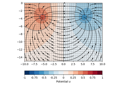
- pygimli.solver.grad(mesh, u, r=None)[source]#
Return the discrete interpolated gradient \(\mathbf{v}\) for a given scalar field \(\mathbf{u}\).
\[\begin{split}\mathbf{v}(\mathbf{r}_{\mathcal{C}}) &= \nabla u(\mathbf{r}_{\mathcal{N}}) \\ (\mathbf{v_x}(\mathbf{r}_{\mathcal{C}}), \mathbf{v_y}(\mathbf{r}_{\mathcal{C}}), \mathbf{v_z}(\mathbf{r}_{\mathcal{C}}))^{\text{T}} &= \left(\frac{\partial u}{\partial x}, \frac{\partial u}{\partial y}, \frac{\partial u}{\partial z}\right)^{\text{T}}\end{split}\]With \(\mathcal{N}=\cup_{i=0}^{N} \text{Node}_i\), \(\mathcal{C}=\cup_{j=0}^{M} \text{Cell}_j\), \(\mathbf{u}=\{u(\mathbf{r}_{i})\}\in I\!R\) and \(\mathbf{r}_{i} = (x_i, y_i, z_i)^{\text{T}}\)
The discrete scalar field \(\mathbf{u}(\mathbf{r}_{\mathcal{N}})\) need to be defined for each node position \(\mathbf{r}_{\mathcal{N}}\). The resulting vector field \(\mathbf{v}(\mathbf{r}_{\mathcal{C}})\) is defined for each cell center position \(\mathbf{r}_{\mathcal{C}}\). If you need other positions than the cell center, provide an appropriate array of coordinates \(\mathbf{r}\).
- Parameters:
mesh (GIMLI::Mesh) – Discretization base, interpolation will be performed via finite element base shape functions.
u (array | callable) – Scalar field per mesh node position or an appropriate callable([[x,y,z]])
r (ndarray((M, 3)) [mesh.cellCenter()]) – Alternative target coordinates :math:`mathbf{r} for the resulting gradient field. i.e., the positions where the vector field is defined. Default are all cell centers.
- Returns:
v – Resulting vector field defined on \(\mathbf{v}(\mathbf{r}_{\mathcal{C}})\). M is number of cells or length of given alternative coordinates r.
- Return type:
ndarray((M, 3))
Examples
>>> import numpy as np
>>> import matplotlib.pyplot as plt
>>> import pygimli as pg
>>> fig, ax = plt.subplots()
>>> mesh = pg.createGrid(x=np.linspace(0, 1, 20), y=np.linspace(0, 1, 20))
>>> u = lambda p: pg.x(p)**2 * pg.y(p)
>>> _ = pg.show(mesh, u(mesh.positions()), ax=ax)
>>> _ = pg.show(mesh, [2.*pg.y(mesh.cellCenters())*pg.x(mesh.cellCenters()),
...             pg.x(mesh.cellCenters())**2], ax=ax)
>>> _ = pg.show(mesh, pg.solver.grad(mesh, u), ax=ax, color='w',
...             linewidth=0.4)
>>> plt.show()

Examples using pygimli.solver.grad
- pygimli.solver.greenDiffusion1D(x, t=0, a=1, dim=1)[source]#
Greens function for diffusion operator.
Provides the elementary solution for:
\[g(x,t) = \partial t + a \Delta\]To find a solution for:
\[u(x,t) \quad\text{for}\quad\frac{\partial u(x,t)}{\partial t} + a \Delta u(x,t) = f(x)\]\[x = [-x, 0, x]\]\[u(x,t) = g(x,t) * f(x)\]- Parameters:
- Returns:
g – Discrete Greens’function
- Return type:
array_like
Examples
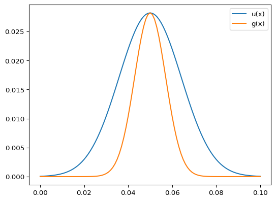
>>> import numpy as np
>>> from pygimli.solver import greenDiffusion1D
>>> dx = 0.001
>>> x = np.arange(0, 0.1+dx, dx)
>>> g = greenDiffusion1D(np.hstack((-x[:0:-1], x)), t=1.0, a=1e-4)
>>> g *= dx
>>> f = np.zeros(len(x))
>>> f[int(len(x)/2)] = 1.
>>> u = np.convolve(g, f)[len(x)-1:2*len(x)-1]
>>> import matplotlib.pyplot as plt
>>> fig, ax = plt.subplots()
>>> _ = ax.plot(x, u, label="u(x)")
>>> _ = ax.plot(x, g[::2], label="g(x)")
>>> _ = ax.legend()
>>> fig.show()
- pygimli.solver.intDomain(u, mesh=None)[source]#
Return integral over nodal solution \(u\).
\[\int_{\Omega} u\]
- pygimli.solver.linSolve(mat, b, solver=None, verbose=False, **kwargs)[source]#
Direct linear solution after \(\textbf{x}\) using core LinSolver.
\[\textbf{A}\textbf{x} = \textbf{b}\]If \(\textbf{A}\) is symmetric, sparse and positive definite.
- Parameters:
mat (GIMLI::RSparseMatrix, GIMLI::RSparseMapMatrix,) –
numpy.array
System matrix. Need to be symmetric, sparse and positive definite.
b (iterable array) – Right hand side of the equation.
solver (str [None]) – Try to choose a solver, ‘pg’ for pygimli core cholmod or umfpack. ‘np’ for numpy linalg or scipy.sparse.linalg. Automatic choosing if solver is None depending on matrixtype.
verbose (bool [False]) – Be verbose.
- Returns:
x – Solution vector.
- Return type:
Examples using pygimli.solver.linSolve
- pygimli.solver.normH1(u, mat=None, mesh=None)[source]#
Create (H1) norm for the finite element space.
- Parameters:
u (iterable) – Node based value to compute the H1 norm for.
mat (Matrix) – Stiffness matrix.
mesh (GIMLI::Mesh) – Mesh with the FE space to generate S if necessary.
- Returns:
ret – \(H1(u)\) norm.
- Return type:
Examples using pygimli.solver.normH1
- pygimli.solver.normL2(u, mat=None, mesh=None)[source]#
Create Lebesgue (L2) norm for finite element space.
Find the L2 Norm for a solution for the finite element space. \(u\) exact solution \({\bf M}\) Mass matrix, i.e., Finite element identity matrix.
\[\begin{split}L2(f(x)) = || f(x) ||_{L^2} & = (\int |f(x)|^2 \mathrm{d}\:x)^{1/2} \\ & \approx h (\sum |f(x)|^2 )^{1/2} \\ L2(u) = || u ||_{L^2} & = (\int |u|^2 \mathrm{d}\:x)^{1/2} \\ & \approx (\sum M (u))^{1/2} \\ e_{L2_rel} = \frac{L2(u)}{L2(u)} & = \frac{(\sum M(u))^{1/2}}{(\sum M u)^{1/2}}\end{split}\]The error for any approximated solution \(u_h\) correlates to the L2 norm of ‘L2Norm(u - u_h, M)’. If you like relative values, you can also normalize this error with ‘L2Norm(u - u_h, M) / L2Norm(u, M)*100’.
- Parameters:
u (iterable) – Node based value to compute the L2 norm for.
mat (Matrix) – Mass element matrix.
mesh (GIMLI::Mesh) – Mesh with the FE space to generate M if necessary.
- Returns:
ret – \(L2(u)\) norm.
- Return type:
Examples using pygimli.solver.normL2
- pygimli.solver.parseArgPairToBoundaryArray(pair, mesh)[source]#
Parse boundary related pair argument to create a list of [ GIMLI::Boundary, value|callable ].
- Parameters:
pair (tuple) –
[marker, arg]
[marker, [callable, *kwargs]]
[marker, [arg_x, arg_y, arg_z]]
[boundary, arg]
[‘*’, arg]
[node, arg]
[[marker, …], arg] (REMOVE ME because of bad design)
[[boundary,…], arg] (REMOVE ME because of bad design)
[marker, callable, *kwargs] (REMOVE ME because of bad design)
[[marker, …], callable, *kwargs] (REMOVE ME because of bad design)
arg will be parsed by
pygimli.solver.solver.generateBoundaryValueand distributed to each boundary. Callable functions will be executed at run time. ‘*’ is interpreted as all boundary elements with one neighboring cellmesh (GIMLI::Mesh) – Used to find boundaries by marker.
- Returns:
bc – [GIMLI::Boundary, value|callable]
- Return type:
list()
- pygimli.solver.parseArgToArray(arg, nDof, mesh=None, userData={})[source]#
Parse array related arguments to create a valid value array.
- Parameters:
arg (float | int | iterable | callable) –
The target array value that will be converted to an array.
If arg is a callable with it must fulfill:
:: arg(cell|node|boundary, userData={})
Where MeshEntity is one of GIMLI::Cell , GIMLI::Node or GIMLI::Boundary depending on nDof, where nDof is mesh.cellCount(), mesh.nodeCount() or mesh.boundaryCount(), respectively.
mesh (GIMLI::Mesh) – Used if arg is callable
userData (class) – Used if arg is callable
- Returns:
ret – Array of desired length filled with the appropriate values.
- Return type:
GIMLI::RVector
Examples using pygimli.solver.parseArgToArray
- pygimli.solver.parseArgToBoundaries(args, mesh)[source]#
Parse boundary related arguments to create a valid boundary value list: [ GIMLI::Boundary, value|callable ]
- Parameters:
args (dict, float, callable) –
Dictionary is preferred (key=value|callable). If args is just a callable or float every outer boundary is processed with args.
List pairs will be removed or not correct parsed for vector valued problems. Callable will be evaluated at runtime. See examples. Else see
pygimli.solver.solver.parseArgPairToBoundaryArraymesh (GIMLI::Mesh) – Used to find boundaries by marker
- Returns:
boundaries – [ GIMLI::Boundary, value|callable ]
- Return type:
list()
Examples
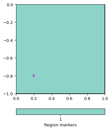
>>> # no need to import matplotlib. pygimli show does
>>> import pygimli as pg
>>> import pygimli.meshtools as mt
>>> plc = mt.createWorld([0, 0], [1, -1], worldMarker=0)
>>> ax, _ = pg.show(plc, boundaryMarker=True)
>>> mesh = mt.createMesh(plc)
>>> # all four outer boundaries get value = 1.0
>>> b = pg.solver.parseArgToBoundaries(1.0, mesh)
>>> print(len(b))
4
>>> # all edges with marker 1 get value = 1.0
>>> b = pg.solver.parseArgToBoundaries({1: 1.0}, mesh)
>>> print(len(b))
1
>>> # same as above with marker 2 get value 2
>>> b = pg.solver.parseArgToBoundaries({'1': 1.0, 2 : 2.0}, mesh)
>>> print(len(b))
2
>>> # same as above with marker 3 get value 3
>>> b = pg.solver.parseArgToBoundaries({1:1., 2:2., 3:3.}, mesh)
>>> print(len(b))
3
>>> # Boundary values for vector valued problem
>>> b = pg.solver.parseArgToBoundaries({1:[1.0, 1.0]}, mesh)
>>> print(len(b), b[0][1])
1 [1.0, 1.0]
>>> # edges with marker 1 and 2 get value 1
>>> b = pg.solver.parseArgToBoundaries({'1,2':1.0}, mesh)
>>> print(len(b))
2
>>> b = pg.solver.parseArgToBoundaries({'1, 2, 3': 1.0}, mesh)
>>> print(len(b))
3
>>> b = pg.solver.parseArgToBoundaries({'1:4':1.0, 4:4.0}, mesh)
>>> print(len(b))
4
>>> b = pg.solver.parseArgToBoundaries({mesh.node(0):0.0}, mesh)
>>> print(len(b))
1
>>> def bCall(boundary):
...     u = []
...     for i, n in enumerate(boundary.nodes()):
...         u.append(i)
...     return u
>>> b = pg.solver.parseArgToBoundaries({1:bCall}, mesh)
>>> print(len(b),b[0][1](b[0][0]))
1 [0, 1]
>>> def bCall(boundary, a1, a2):
...     return a1 + a2
>>> b = pg.solver.parseArgToBoundaries({1: [bCall, {'a1':2, 'a2':3}]}, mesh)
>>> print(len(b), b[0][1][0](b[0][0], **b[0][1][1]))
1 5
>>> b = pg.solver.parseArgToBoundaries({1: [bCall, {'a1':1, 'a2':2}],
...                                     2: [bCall, {'a1':3, 'a2':4}]}, mesh)
>>> print(len(b), b[0][1][0](b[0][0], **b[0][1][1]))
2 3
>>> b = pg.solver.parseArgToBoundaries({'1,2': [bCall, {'a1':4, 'a2':5}]}, mesh)
>>> print(len(b), b[1][1][0](b[1][0], **b[1][1][1]))
2 9
>>> pg.wait()

Examples using pygimli.solver.parseArgToBoundaries
- pygimli.solver.parseMapToCellArray(attributeMap, mesh, default=0.0)[source]#
Parse a value map to cell attributes.
A map should consist of pairs of marker and value. A marker is an integer and corresponds to the cell.marker().
- Parameters:
mesh (GIMLI::Mesh) – For each cell of mesh a value will be returned.
attributeMap (list | dict) – List of pairs [marker, value] ] || [[marker, value]], or dictionary with marker keys
default (float [0.0]) – Fill all unmapped attributes to this default.
- Returns:
att – Array of length mesh.cellCount()
- Return type:
array
Examples using pygimli.solver.parseMapToCellArray
- pygimli.solver.parseMarkersDictKey(key, markers)[source]#
Parse dictionary key of type str to marker list.
Utility function to parse a dictionary key string into a valid list of markers containing in a given markers list.
- Parameters:
- Returns:
mas – List of integers described by key
- Return type:
[int]
- pygimli.solver.showSparseMatrix(mat, full=False)[source]#
Show the content of a sparse matrix.
- Parameters:
mat (GIMLI::SparseMatrix | GIMLI::SparseMapMatrix) – Matrix to be shown.
full (bool [False]) – Show as dense matrix.
- pygimli.solver.solve(mesh, **kwargs)[source]#
Solve partial differential equation.
This is a syntactic sugar convenience function for solving partial differential equation on a given mesh. Using the best guess method for the given parameter. Currently only Finite Element calculation using
pygimli.solver.solveFiniteElements
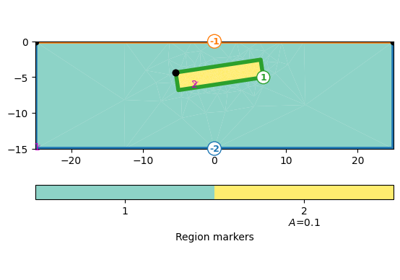
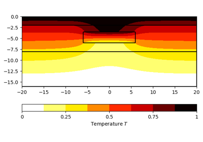
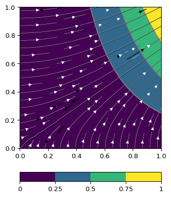
- pygimli.solver.solveFiniteElements(mesh, a=1.0, b=None, f=0.0, bc=None, times=None, c=1.0, userData={}, verbose=False, **kwargs)[source]#
Solve partial differential equation with Finite Elements.
This is a syntactic sugar convenience function for using the Finite Element functionality of the library core to solve partial differential equation (PDE) that match the following form:
\[\begin{split}c \frac{\partial u}{\partial t} & = \nabla\cdot(a \nabla u) + b u + f(\mathbf{r},t)~~|~~\Omega_{\text{Mesh}}\\ u & = h~~|~~\Gamma_{\text{Dirichlet}}\\ a\frac{\partial u}{\partial \mathbf{n}} & = g~~|~~\Gamma_{\text{Neumann}}\\ \alpha u + \beta\frac{\partial u}{\partial \mathbf{n}} & = \gamma~~|~~\Gamma_{\text{Robin}}\\ \frac{\partial u}{\partial \mathbf{n}} & = \alpha(u_0-u)~~|~~\Gamma_{\text{Robin}}\end{split}\]for the scalar \(u(\mathbf{r}, t)\) or vector \(\mathbf(u)(\mathbf{r}, t)\) solution at each node of a given mesh. The Domain \(\Omega\) and the Boundary \(\Gamma\) are defined through the mesh with appropriate boundary marker.
To ensure vector solution, either set vector forces or at least one vector component boundary condition.
- Parameters:
mesh (GIMLI::Mesh) – Mesh represents spatial discretization of the calculation domain
a (value | array | callable(cell, userData)) – Cell values of type float or complex can be scalar, anisotropy matrix or elastic tensor.
b (value | array | callable(cell, userData) [None]) – Cell values. None means the term is unused.
c (value | array | callable(cell, userData) [None]) – Scale the unsteady term, only for times is not None.
f (value | array(cells) | array(nodes) | callable(args, kwargs)) – force values, for vector fields use (n x dim) values.
bc (dict()) –
Dictionary of boundary conditions. Current supported boundary conditions by dictionary keys: ‘Dirichlet’, ‘Neumann’, ‘Robin’, ‘Node’.
The dictionary can contain multiple “key: Arg” Arg will be parsed by
pygimli.solver.solver.parseArgPairToBoundaryArrayIf the dictionary key is ‘Node’ then fixed values for single node indices can by be given. e.g., bc={‘Node’: [nodeID, value]}. Note this is only a shortcut for bc={‘Dirichlet’: [mesh.node(nodeID), value]}.
The parameter $a$ for Neumann boundary condition is choosen automatically from the diffusivity parameter $a$ of the associated cell.
times (array [None]) – Solve as time dependent problem for the given times.
- Keyword Arguments:
**kwargs –
- u0: value | array | callable(pos, userData)
Node values
- theta: float [1]
\(theta = 0\) means explicit Euler, maybe stable for
\(\Delta t \quad\text{near}\quad h\) * \(theta = 0.5\), Crank-Nicolson scheme, maybe instable * \(theta = 2/3\), Galerkin scheme * \(theta = 1\), implicit Euler
If unsure choose \(\theta = 0.5 + \epsilon\) (probably stable).
- dynamic: bool [False]
Boundary conditions for time depending problems will be considered dynamic for each time step.
- stats: bool
Give some statistics.
- progress: bool
Give some calculation progress.
- assembleOnly: bool
Stops after matrix asssemblation. Returns the system matrix A and the rhs vector.
- fixPureNeumann: bool [auto]
If set or detected automatic, we add the additional condition: \(\int_\Omega u dv = 0\) making elliptic problems well-posed.
- rhs: iterable
Pre assembled rhs. Will preferred on any f settings.
- ws: dict
The WorkSpace is a dictionary that will get some temporary data during the calculation. Any keyvalue ‘u’ in the dictionary is used for the resulting array.
- vectorValued: bool (False)
Solution forced to vector valued, in case the auto detection fails
- Returns:
u – Returns the solution u either 1,n array for stationary problems or for m,n array for m time steps
- Return type:
array
See also
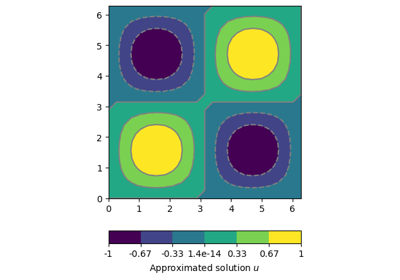
Examples
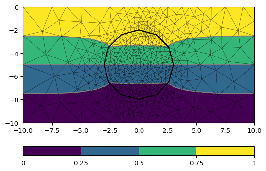
>>> # no need to import matplotlib, pygimli show does.
>>> import pygimli as pg
>>> import pygimli.meshtools as mt
>>> world = mt.createWorld(start=[-10, 0], end=[10, -10],
...                        marker=1, worldMarker=False)
>>> c1 = mt.createCircle(pos=[0.0, -5.0], radius=3.0, area=.1, marker=2)
>>> mesh = mt.createMesh([world, c1], quality=34.3)
>>> u = pg.solver.solveFiniteElements(mesh, a={1: 100.0, 2: 1.0},
...                                   bc={'Dirichlet':{4: 1.0, 3: 0.0}})
>>> ax = pg.show(mesh, u, showMesh=True)[0]
>>> _ = pg.show(c1, ax=ax, fillRegion=False)

Examples using pygimli.solver.solveFiniteElements
- pygimli.solver.solveFiniteVolume(mesh, a=1.0, b=0.0, f=0.0, fn=0.0, vel=None, u0=0.0, times=None, uL=None, relax=1.0, ws=None, scheme='CDS', **kwargs)[source]#
Solve partial differential equation with Finite Volumes.
This function is a syntactic sugar proxy for using the Finite Volume functionality of the library core to solve elliptic and parabolic partial differential of the following type:
\[\begin{split}\frac{\partial u}{\partial t} + \mathbf{v}\cdot\nabla u & = \nabla\cdot(a \nabla u) + b u + f(\mathbf{r},t)\\ u(\mathbf{r}, t) & = u_B \quad\mathbf{r}\in\Gamma_{\text{Dirichlet}}\\ \frac{\partial u(\mathbf{r}, t)}{\partial \mathbf{n}} & = u_{\partial \text{B}} \quad\mathbf{r}\in\Gamma_{\text{Neumann}}\\ u(\mathbf{r}, t=0) & = u_0 \quad\text{with} \quad\mathbf{r}\in\Omega\end{split}\]The Domain \(\Omega\) and the Boundary \(\Gamma\) are defined through the given mesh with appropriate boundary marker.
The solution \(u(\mathbf{r}, t)\) is given for each cell in the mesh.
- Parameters:
mesh (GIMLI::Mesh) – Mesh represents spatial discretization of the calculation domain
a (value | array | callable(cell, userData)) – Stiffness weighting per cell values.
b (value | array | callable(cell, userData)) – Scale for mass values b
f (iterable(cell)) – Load vector
fn (iterable(cell)) – TODO What is fn
vel (ndarray (N,dim) | RMatrix(N,dim)) – Velocity field \(\mathbf{v}(\mathbf{r}, t=\text{const}) = \{[v_i]_j,\}\) with \(i=[1\ldots 3]\) for the mesh dimension and \(j = [0\ldots N-1]\) with N either the amount of cells, nodes, or boundaries. Velocities per boundary are preferred and will be interpolated on demand.
u0 (value | array | callable(cell, userData)) – Starting field
times (iterable) – Time steps to calculate for.
Workspace (ws) –
This can be an empty class that will used as an Workspace to store and cache data.
If ws is given: The system matrix is taken from ws or calculated once and stored in ws for further usage.
The system matrix is cached in this Workspace as ws.S The LinearSolver with the factorized matrix is cached in this Workspace as ws.solver The rhs vector is only stored in this Workspace as ws.rhs
scheme (str [CDS]) – Finite volume scheme:
pygimli.solver.diffusionConvectionKernel**kwargs –
bc : Boundary Conditions dictionary, see pg.solver
uB : Dirichlet boundary conditions DEPRECATED
duB : Neumann boundary conditions DEPRECATED
- Returns:
u – Solution field for all time steps.
- Return type:
ndarray(nTimes, nCells)
Examples using pygimli.solver.solveFiniteVolume
Classes#
- class pygimli.solver.LinSolver(mat=None, solver=None, verbose=False, **kwargs)[source]#
Bases:
objectProxy class for the solution of linear systems of equations.
- class pygimli.solver.RungeKutta(solver, verbose=False)[source]#
Bases:
objectTODO DOCUMENT ME
- rk4a = [0.0, -0.41789047449985195, -1.192151694642677, -1.6977846924715279, -1.5141834442571558]#
- rk4b = [0.14965902199922912, 0.37921031299962726, 0.8229550293869817, 0.6994504559491221, 0.15305724796815198]#
- rk4c = [0.0, 0.14965902199922912, 0.37040095736420475, 0.6222557631344432, 0.9582821306746903]#