Note
Go to the end to download the full example code
Naive complex-valued electrical inversion#
This example presents a quick and dirty proof-of-concept for a complex-valued inversion, similar to Kemna, 2000. The normal equations are solved using numpy, and no optimization with respect to running time and memory consumptions are applied. As such this example is only a technology demonstration and should not be used for real-world inversion of complex resistivity data!
Kemna, A.: Tomographic inversion of complex resistivity – theory and application, Ph.D. thesis, Ruhr-Universität Bochum, doi:10.1111/1365-2478.12013, 2000.
Note
This is a technology demonstration. Don’t use this code for research. If you require a complex-valued inversion, please contact us at info@pygimli.org
import numpy as np
import matplotlib.pyplot as plt

import pygimli as pg
import pygimli.meshtools as mt
from pygimli.physics import ert
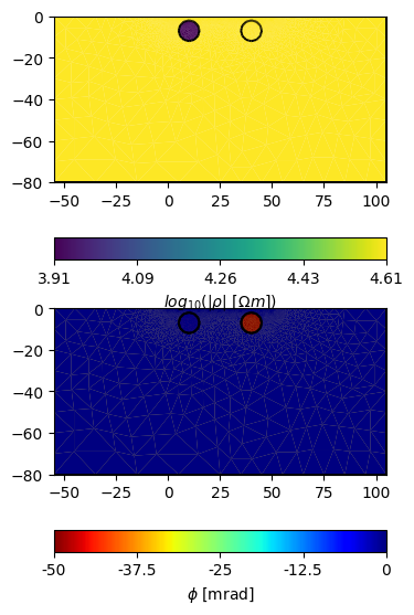
For reference we later plot the true complex resistivity model as reference
def get_scheme():
"""Create data scheme of dipole-dipole array."""
scheme = ert.createData(elecs=np.linspace(start=0, stop=50, num=51),
schemeName='dd')
# Not strictly required, but we switch potential electrodes to yield
# positive geometric factors. Note that this was also done for the
# synthetic data inverted later.
m = scheme['m']
n = scheme['n']
scheme['m'] = n
scheme['n'] = m
scheme.set('k', [1 for x in range(scheme.size())])
return scheme
def get_fwd_mesh():
"""Generate the forward mesh (with embedded anomalies)."""
scheme = get_scheme()
# Mesh generation
world = mt.createWorld(
start=[-55, 0], end=[105, -80], worldMarker=True)
conductive_anomaly = mt.createCircle(
pos=[10, -7], radius=5, marker=2
)
polarizable_anomaly = mt.createCircle(
pos=[40, -7], radius=5, marker=3
)
plc = mt.mergePLC((world, conductive_anomaly, polarizable_anomaly))
# local refinement of mesh near electrodes
for s in scheme.sensors():
plc.createNode(s + [0.0, -0.2])
mesh_coarse = mt.createMesh(plc, quality=33)
mesh = mesh_coarse.createH2()
return mesh
def generate_forward_data():
"""Generate synthetic forward data that we then invert."""
scheme = get_scheme()
mesh = get_fwd_mesh()
rhomap = [
[1, pg.utils.complex.toComplex(100, 0 / 1000)],
# Magnitude: 50 ohm m, Phase: -50 mrad
[2, pg.utils.complex.toComplex(50, 0 / 1000)],
[3, pg.utils.complex.toComplex(100, -50 / 1000)],
]
rho = pg.solver.parseArgToArray(rhomap, mesh.cellCount(), mesh)
fig, axes = plt.subplots(2, 1, figsize=(16 / 2.54, 16 / 2.54))
pg.show(
mesh,
data=np.log(np.abs(rho)),
ax=axes[0],
label=r"$log_{10}(|\rho|~[\Omega m])$"
)
pg.show(mesh, data=np.abs(rho), ax=axes[1], label=r"$|\rho|~[\Omega m]$")
pg.show(
mesh, data=np.arctan2(np.imag(rho), np.real(rho)) * 1000,
ax=axes[1],
label=r"$\phi$ [mrad]",
cMap='jet_r'
)
data = ert.simulate(
mesh,
res=rhomap,
scheme=scheme,
# noiseAbs=0.0,
# noiseLevel=0.0,
)
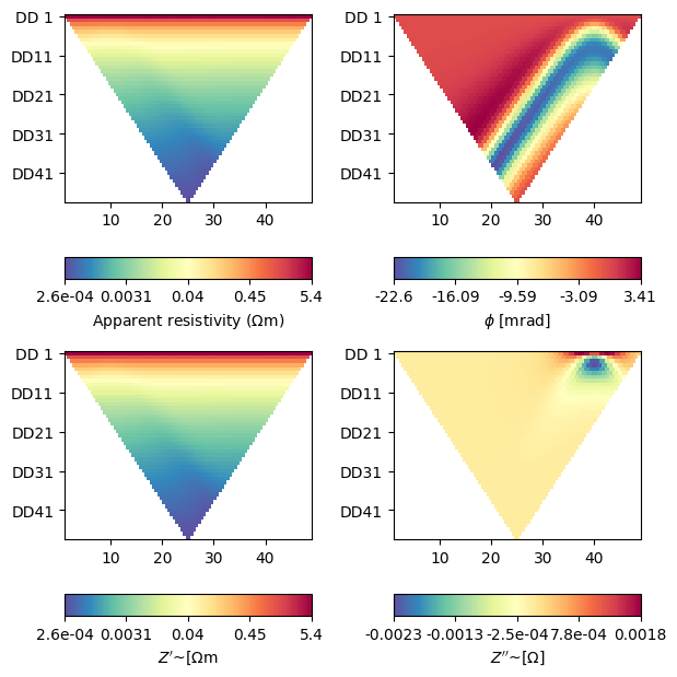
r_complex = data['rhoa'].array() * np.exp(1j * data['phia'].array())
# Please note the apparent negative (resistivity) phases!
fig, axes = plt.subplots(2, 2, figsize=(16 / 2.54, 16 / 2.54))
ert.showERTData(data, vals=data['rhoa'], ax=axes[0, 0])
# phia is stored in radians, but usually plotted in milliradians
ert.showERTData(
data, vals=data['phia'] * 1000, label=r'$\phi$ [mrad]', ax=axes[0, 1])
ert.showERTData(
data, vals=np.real(r_complex), ax=axes[1, 0],
label=r"$Z'$~[$\Omega$m"
)
ert.showERTData(
data, vals=np.imag(r_complex), ax=axes[1, 1],
label=r"$Z''$~[$\Omega$]"
)
fig.tight_layout()
fig.show()
return r_complex
data_rcomplex = generate_forward_data()
def plot_fwd_model(axes):
"""Plot the forward model used to generate the data."""
# Mesh generation
world = mt.createWorld(
start=[-55, 0], end=[105, -80], worldMarker=True)
conductive_anomaly = mt.createCircle(
pos=[10, -7], radius=5, marker=2
)
polarizable_anomaly = mt.createCircle(
pos=[40, -7], radius=5, marker=3
)
plc = mt.mergePLC((world, conductive_anomaly, polarizable_anomaly))
# local refinement of mesh near electrodes
for s in scheme.sensors():
plc.createNode(s + [0.0, -0.2])
mesh_coarse = mt.createMesh(plc, quality=33)
mesh = mesh_coarse.createH2()
rhomap = [
[1, pg.utils.complex.toComplex(100, 0 / 1000)],
# Magnitude: 50 ohm m, Phase: -50 mrad
[2, pg.utils.complex.toComplex(50, 0 / 1000)],
[3, pg.utils.complex.toComplex(100, -50 / 1000)],
]
rho = pg.solver.parseArgToArray(rhomap, mesh.cellCount(), mesh)
pg.show(
mesh,
data=np.log(np.abs(rho)),
ax=axes[0],
label=r"$log_{10}(|\rho|~[\Omega m])$"
)
pg.show(mesh, data=np.abs(rho), ax=axes[1], label=r"$|\rho|~[\Omega m]$")
pg.show(
mesh, data=np.arctan2(np.imag(rho), np.real(rho)) * 1000,
ax=axes[2],
label=r"$\phi$ [mrad]",
cMap='jet_r'
)
fig.tight_layout()
fig.show()
Create a measurement scheme for 51 electrodes, spacing 1
scheme = ert.createData(elecs=np.linspace(start=0, stop=50, num=51),
                        schemeName='dd')
# Not strictly required, but we switch potential electrodes to yield positive
# geometric factors. Note that this was also done for the synthetic data
# inverted later.
m = scheme['m']
n = scheme['n']
scheme['m'] = n
scheme['n'] = m
scheme['k'] = np.ones(scheme.size())
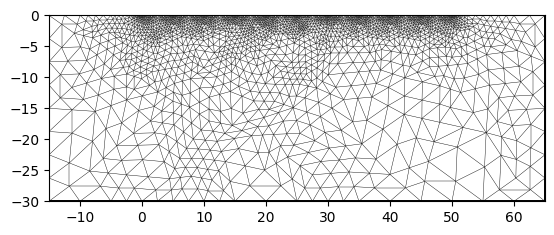
Mesh generation for the inversion
world = mt.createWorld(
    start=[-15, 0], end=[65, -30], worldMarker=False, marker=2)

# local refinement of mesh near electrodes
for s in scheme.sensors():
    world.createNode(s + [0.0, -0.4])

mesh_coarse = mt.createMesh(world, quality=33)
mesh = mesh_coarse.createH2()
for nr, c in enumerate(mesh.cells()):
    c.setMarker(nr)
pg.show(mesh)
(<Axes: >, None)
Define start model of the inversion [magnitude, phase]
start_model = np.ones(mesh.cellCount()) * pg.utils.complex.toComplex(
    80, -0.01 / 1000)
Initialize the complex forward operator
fop = ert.ERTModelling(
    sr=False,
    verbose=True,
)
fop.setComplex(True)
fop.setData(scheme)
fop.setMesh(mesh, ignoreRegionManager=True)
fop.mesh()
Mesh: Nodes: 2373 Cells: 4472 Boundaries: 6844
Compute response for the starting model
Regularization matrix
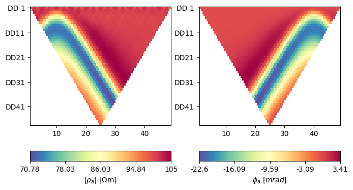
read-in data and determine error parameters filename = pg.getExampleFile(
‘CR/synthetic_modeling/data_rre_rim.dat’, load=False, verbose=True)
data_rre_rim = np.loadtxt(filename) N = int(data_rre_rim.size / 2) d_rcomplex = data_rre_rim[:N] + 1j * data_rre_rim[N:]
N = data_rcomplex.shape[0]
dmag = np.abs(data_rcomplex)
dpha = np.arctan2(data_rcomplex.imag, data_rcomplex.real) * 1000

fig, axes = plt.subplots(1, 2, figsize=(20 / 2.54, 10 / 2.54))
k = np.array(ert.createGeometricFactors(scheme))
ert.showERTData(
    scheme, vals=dmag * k, ax=axes[0], label=r'$|\rho_a|~[\Omega$m]')
ert.showERTData(scheme, vals=dpha, ax=axes[1], label=r'$\phi_a~[mrad]$')

# real part: log-magnitude
# imaginary part: phase [rad]
d_rlog = np.log(data_rcomplex)

# add some noise
np.random.seed(42)

noise_magnitude = np.random.normal(
    loc=0,
    scale=np.exp(d_rlog.real) * 0.04
)

# absolute phase error
noise_phase = np.random.normal(
    loc=0,
    scale=np.ones(N) * (0.5 / 1000)
)

d_rlog = np.log(np.exp(d_rlog.real) + noise_magnitude) + 1j * (
    d_rlog.imag + noise_phase)

# crude error estimations
rmag_linear = np.exp(d_rlog.real)
err_mag_linear = rmag_linear * 0.04 + np.min(rmag_linear)
err_mag_log = np.abs(1 / rmag_linear * err_mag_linear)

Wd = np.diag(1.0 / err_mag_log)
WdTwd = Wd.conj().dot(Wd)
Put together one iteration of a naive inversion in log-log transformation d = log(V) m = log(sigma)
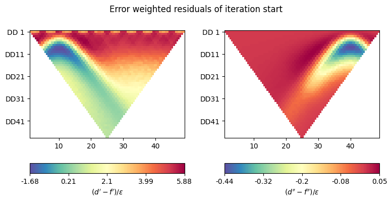
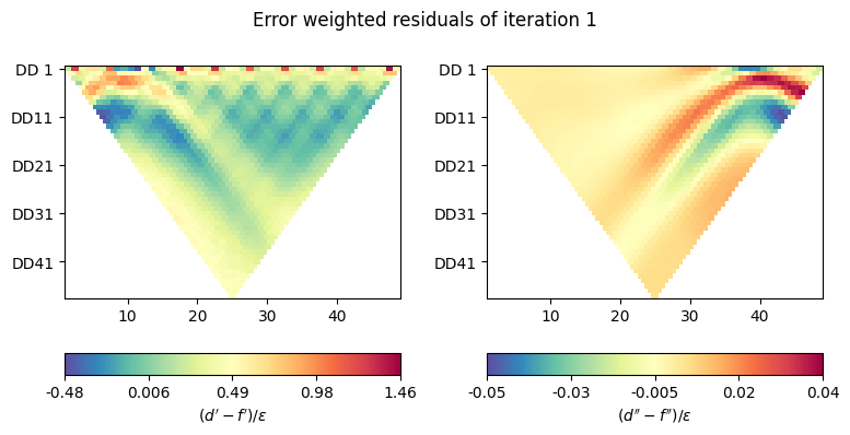
def plot_inv_pars(filename, d, response, Wd, iteration='start'):
    """Plot error-weighted residuals."""
    if 0:
        fig, axes = plt.subplots(1, 1, figsize=(20 / 2.54, 10 / 2.54))

        psi = np.abs(Wd.dot(d - response))

        ert.showERTData(
            scheme, vals=psi, ax=axes,
            label=r"$(d' - f') / \epsilon$"
        )
    else:
        fig, axes = plt.subplots(1, 2, figsize=(20 / 2.54, 10 / 2.54))
        psi = Wd.dot(d - response)
        ert.showERTData(
            scheme, vals=psi.real, ax=axes[0],
            label=r"$(d' - f') / \epsilon$"
        )
        ert.showERTData(
            scheme, vals=psi.imag, ax=axes[1],
            label=r"$(d'' - f'') / \epsilon$"
        )

        fig.suptitle(f'Error weighted residuals of iteration {iteration}',
                     y=1.0)

    fig.tight_layout()


m_old = np.log(start_model)
# d = np.log(pg.utils.toComplex(data_rre_rim))
d = np.log(data_rcomplex)
response = np.log(pg.utils.toComplex(f_0))
# tranform to log-log sensitivities
J = J0 / np.exp(response[:, np.newaxis]) * np.exp(m_old)[np.newaxis, :]
lam = 100

plot_inv_pars('stats_it0.jpg', d, response, Wd)

# only one iteration is implemented here!
for i in range(1):
    print('-' * 80)
    print('Iteration {}'.format(i + 1))

    term1 = J.conj().T.dot(WdTwd).dot(J) + lam * Wm.T.dot(Wm)
    # term1_inverse = np.linalg.inv(term1)
    term2 = J.conj().T.dot(WdTwd).dot(d - response) - lam * Wm.T.dot(Wm).dot(
        m_old)
    # model_update = term1_inverse.dot(term2)
    model_update = np.linalg.solve(
        term1,
        term2
    )

    print('Model Update')
    print(model_update)

    m1 = np.array(m_old + 1.0 * model_update).squeeze()
--------------------------------------------------------------------------------
Iteration 1
Model Update
[0.19006749-7.60207166e-05j 0.18687016-5.68031681e-05j
 0.19731258-1.17414927e-04j ... 0.11804832-1.64495115e-03j
 0.11011347-1.67094449e-03j 0.11465995-1.66143964e-03j]
Now plot the residuals for the first iteration
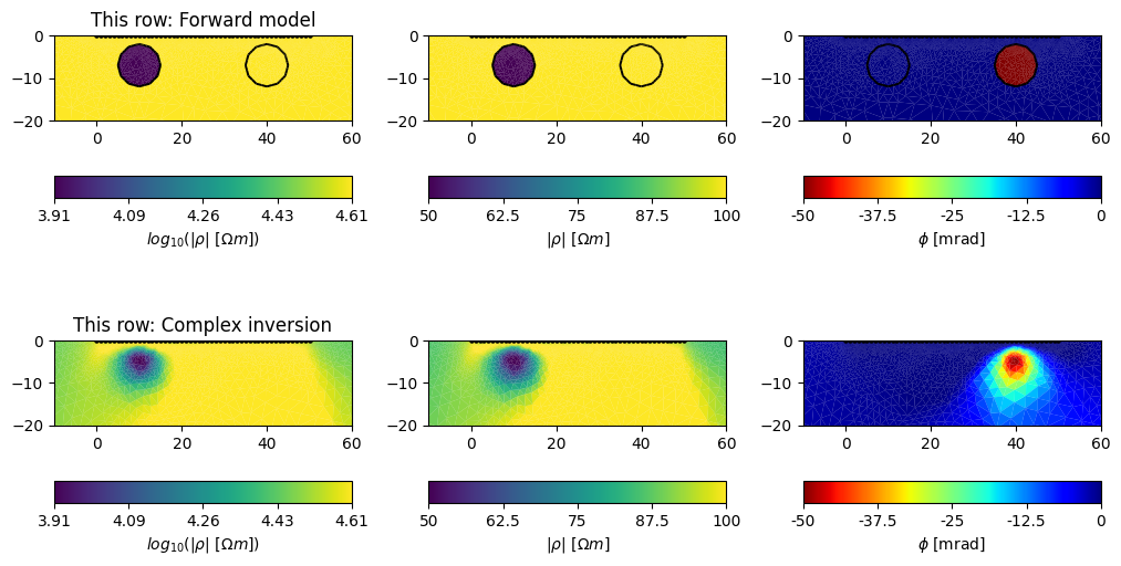
And finally, plot the inversion results
fig, axes = plt.subplots(2, 3, figsize=(26 / 2.54, 15 / 2.54))
plot_fwd_model(axes[0, :])
axes[0, 0].set_title('This row: Forward model')

pg.show(
    mesh, data=m1.real, ax=axes[1, 0],
    cMin=np.log(50),
    cMax=np.log(100),
    label=r"$log_{10}(|\rho|~[\Omega m])$"
)
pg.show(
    mesh, data=np.exp(m1.real), ax=axes[1, 1],
    cMin=50, cMax=100,
    label=r"$|\rho|~[\Omega m]$"
)
pg.show(
    mesh, data=m1.imag * 1000, ax=axes[1, 2], cMap='jet_r',
    label=r"$\phi$ [mrad]",
    cMin=-50, cMax=0,
)

axes[1, 0].set_title('This row: Complex inversion')

for ax in axes.flat:
    ax.set_xlim(-10, 60)
    ax.set_ylim(-20, 0)
    for s in scheme.sensors():
        ax.scatter(s[0], s[1], color='k', s=5)

fig.tight_layout()
Total running time of the script: (0 minutes 56.650 seconds)