Flexible mesh generation using Gmsh

In this example, we learn how to define arbitrary geometries, boundaries, and regions using an external mesh generator (Gmsh).

Task:

Construct a mesh with arbitrary geometry, boundaries and regions for computations in GIMLi.

Problem:

For complex geometries, mesh construction using the poly tools can be cumbersome and lacks of straightforward visual inspection.

Solution:

Create the mesh in Gmsh, a 3D finite element mesh generator with parametric input and advanced visualization capabilities, and convert it to GIMLi for subsequent modelling and inversion.

When the scientific task requires a complex finite-element discretization (i.e. incorporation of structural information, usage of a complete electrode model (CEM), etc.), external meshing tools with visualization capabilities may be the option of choice for some users. In general, the bindings provided by pygimli allow to interface any external mesh generation software.

This HowTo presents an example using Gmsh [Geuzaine and Remacle, 2009]. Gmsh allows for parametric input, i.e. physical boundaries and regions (and any other input) can be specified interactively using the graphical user interface or Gmsh’s own scripting language. A lot of profound tutorials can be found on the Gmsh website (http://www.gmsh.info) or elsewhere. Here, a crosshole ERT example with geological a priori information is presented with a focus on the usage in GIMLi.

Geometry

We start with the definition of several points to layout the main geometry. A point is created via the graphical user interface as illustrated in the following figure.

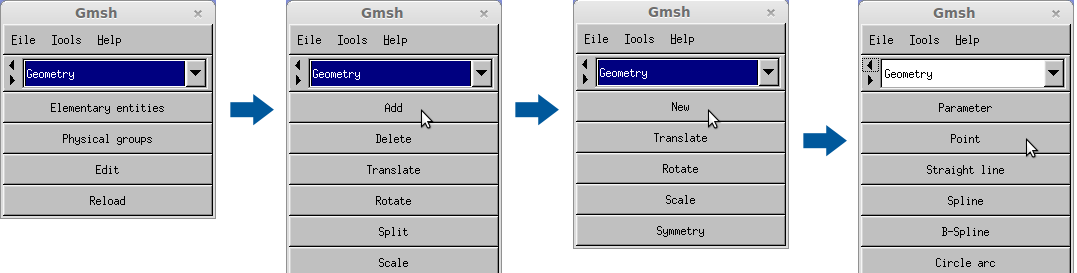
Steps to create a point via the graphical user interface.

We create a large domain to solve the forward problem and specify the coordinates as well as a characteristic length to constrain the relative size of the mesh elements at that point (this is also useful for near-electrode refinement for example).

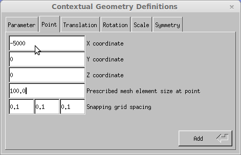
Setting the parameters of a point.

In the geometry file being created, this step would correspond the following command.

Point(1) = {-5000, 0, 0, cl1};

During this HowTo, we will switch between the GUI input and the scripting language. Gmsh’s reload button allows for quick and straightforward interaction between both modes.

Note that it is convenient to replace the characteristic length by a variable During this HowTo, we will switch between the GUI input and the scripting language. Subsequent to the definition of the corner points, we can set up the boundaries by connecting the points created, as shown below.

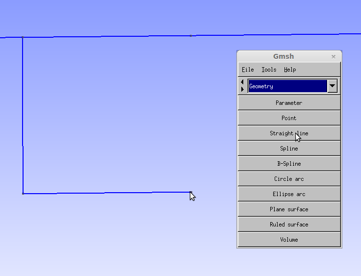
Connecting geometric points using straight lines.

The corresponding command in the script to connect points 1 and 5 would look like this:

Line(1) = {1, 5};

Obviously, we also have to define the electrode positions:

For i In {0:9}
Point(newp) = {15,0,-4*(i+2),cl2}; // Borehole 1
Point(newp) = {35,0,-4*(i+2),cl2}; // Borehole 2
EndFor

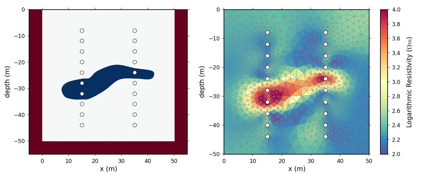
Similarly, we define a set of points describing a geological body and connect them with a spline curve:

Spline(100) = {31, 32, 33, 34, 35, 36, 37, 38, 39, 40,
            41, 42, 43, 44, 45, 29, 30, 31};

After the definition of all points and lines, we can define the three surfaces. A surface is created by selecting Plane Surface from the menu and clicking on the bounding lines and the holes (if present). The following figure illustrates the definition of the outer surface.

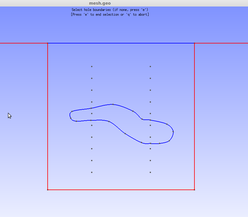
Creating a surface by clicking on the boundaries.

When the surfaces (or volumes in 3D) have been defined, the mesh can be generated by simply clicking the 2D button in the mesh menu (Mesh - 2D). As you will notice, the electrodes are not located on node points, as they # do not layout any geometric feature. To change this, we can embed them in the surfaces (Mesh - Define - Embedded Points) or directly in the script via:

Point{10, 12, 14, ..., 17, 23, 25, 27} In Surface{106};
Point{18, 19, 21} In Surface{104}; // electrodes within the target

Boundaries and regions

Since Gmsh allows for parametric input, we can finally specify the boundary conditions and region marker. This is done in the Physical Groups section under Geometry. The group numbers can be changed within the script. Number 1 is assigned to a Neumann-type boundary condition and number 2 to a mixed one.

Physical Line(1) = {3, 2, 1}; // Free surface
Physical Line(2) = {4, 5, 6}; // Mixed boundary conditions

The indices of the regions will directly map to the region marker in BERT.

Physical Surface(1) = {102}; // Outer region
Physical Surface(2) = {106}; // Inversion region
Physical Surface(3) = {104}; // Geological body

Finally, we assign all electrodes to a Physical Group with the marker 99.

Physical Point(99) = {9, 11, ..., 24, 26, 28}; // electrode marker (99)

That’s it! Now, you can re-run the meshing algorithm and save the result.

Note that in addition to the characteristic length at each point, there are many different ways to constrain the element size (in general or locally) and the resulting mesh quality, which will not be discussed here.

The final geometry can be downloaded here and meshed in the GUI or via the command:

gmsh -2 -o mesh.msh mesh.geo

Import to GIMLi

Any Gmsh output (2D and 3D) can be imported using pygimli and subsequently saved to the binary format.

import subprocess

import matplotlib.pyplot as plt

import pygimli as pg
from pygimli.meshtools import readGmsh


filename = pg.getExampleFile("gmsh/2d_tutorial.geo")

try:
    subprocess.call(
        ["gmsh", "-format", "msh2", "-2", "-o", "mesh.msh", filename])
    gmsh = True
except OSError:
    print("Gmsh needs to be installed for this example.")
    gmsh = False

fig, ax = plt.subplots()
if gmsh:
    mesh = readGmsh("mesh.msh", verbose=True)
    pg.show(mesh, ax=ax, markers=True, clipBoundaryMarkers=True)
    ax.set_xlim(-3, 53)
    ax.set_ylim(-53, 3)
else:
    ax.set_title("Gmsh needs to be installed for this example")
pg.wait()

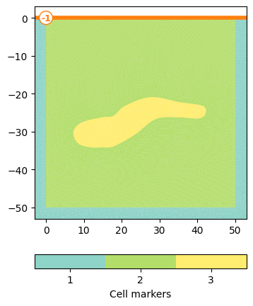
Reading mesh.msh...

  Nodes: 11387
  Entries: 22792
    Points: 20
    Lines: 220
    Triangles: 22552
    Quads: 0
    Tetrahedra: 0

Creating mesh object...

  Dimension: 2-D
  Boundary types: 2 (-2, -1)
  Regions: 3 (1, 2, 3)
  Marked nodes: 20 (99,)

Done.

  Mesh: Nodes: 11387 Cells: 22552 Boundaries: 33938

Synthetic example.

For the sake of illustration, the example presented was chosen to be simple and two-dimensional, although Gmsh and the import function provided allow for much more…

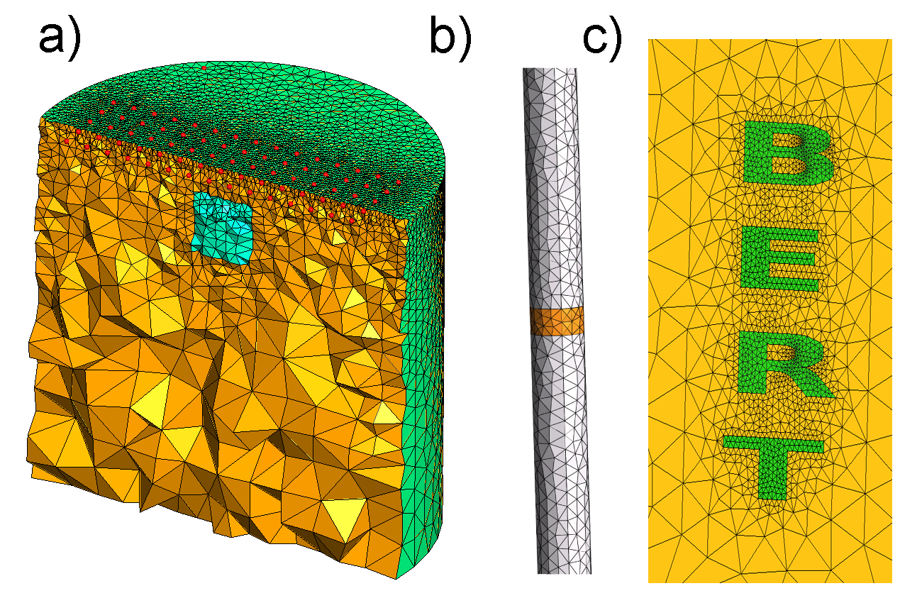
Additional Gmsh examples: a) Laboratory sandbox model. b) Finite discretization of a ring-shaped electrode. c) And more!