2D gravity modelling and inversion

In the following, we will build the model, create synthetic data, and do inversion using a depth-weighting function as outlined in the paper.

import numpy as np
import pygimli as pg
import pygimli.meshtools as mt
# from pygimli.viewer import pv
from pygimli.physics.gravimetry import GravityModelling2D

Synthetic model and data generation

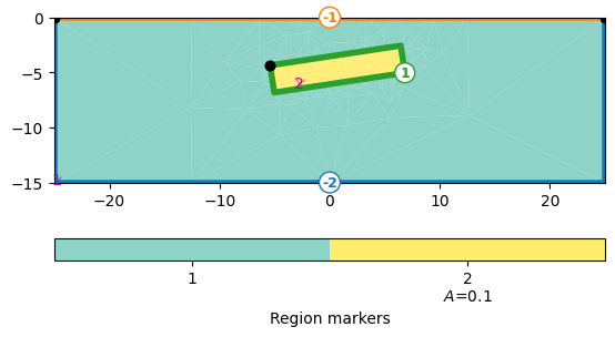
We create a rectangular modelling domain (50x15m) with a flat anomaly in a depth of about 5m.

world = mt.createWorld(start=[-25, 0], end=[25, -15],
                       marker=1)
rect = mt.createRectangle(start=[-6, -3.5], end=[6, -6.0],
                          marker=2, area=0.1)
rect.rotate([0, 0, 0.15])

geom = world + rect
pg.show(geom, markers=True)
mesh = mt.createMesh(geom, quality=33, area=0.2)

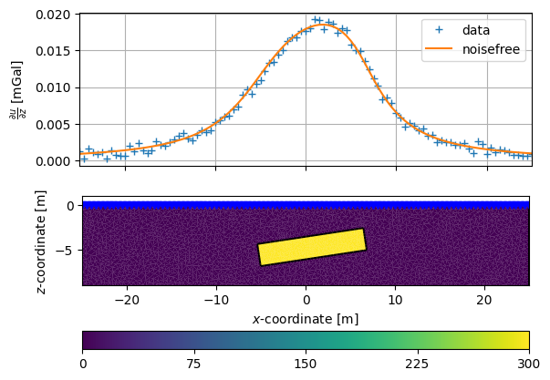
We assume measuring the gravity on a 50m long profile with dense spacing. We initialize the forward response by passing mesh and measuring points. Additionally, we map a density to the cell markers to build a model vector.

x = np.arange(-25, 25.1, .5)
pnts = np.array([x, np.zeros(len(x))]).T

fop = GravityModelling2D(mesh=mesh, points=pnts)
dRho = pg.solver.parseMapToCellArray([[1, 0.0], [2, 300]], mesh)
g = fop.response(dRho)

We define an absolute error and add some Gaussian noise.

error = 0.0005
data = g + np.random.randn(len(g)) * error

The model response is then plotted along with the model

fig, ax = pg.plt.subplots(ncols=1, nrows=2, sharex=True)
ax[0].plot(x, data, "+", label="data")
ax[0].plot(x, g, "-", label="noisefree")
ax[0].set_ylabel(r'$\frac{\partial u}{\partial z}$ [mGal]')
ax[0].grid()
ax[0].legend()

pg.show(mesh, dRho, ax=ax[1])
ax[1].plot(x, x*0, 'bv')
ax[1].set_xlabel('$x$-coordinate [m]')
ax[1].set_ylabel('$z$-coordinate [m]')
ax[1].set_ylim((-9, 1))
ax[1].set_xlim((-25, 25))

(-25.0, 25.0)

For inversion, we create a new mesh from the rectangular domain and setup a new instance of the modelling operator.

mesh = mt.createMesh(world, quality=33, area=1)
fop = GravityModelling2D(mesh=mesh, points=pnts)

Depth weighting

In the paper of Li & Oldenburg (1996), they propose a depth weighting of the constraints with the formula

\[w_z = \frac{1}{(z+z_0)^{3/2}}\]

cz = -pg.y(mesh.cellCenters())
z0 = 5
wz = 1 / (cz+z0)**1.5
pg.show()[0].plot(cz, wz, ".")

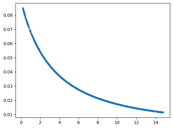
[<matplotlib.lines.Line2D object at 0x7fe735841990>]

Inversion

For inversion, we use geostatistic regularization with a higher correlation length for x, compared to y, to account for the large equivalence. We limit the model to reasonable density contrasts of +/- 1000 kg/m^3. As the depth weighting decreases the local regularization weights, we have to increase the overall regularization strength lambda.

fop.region(1).setConstraintType(2)
inv = pg.Inversion(fop=fop)
inv.setRegularization(limits=[-1000, 1000], trans="Cot",
                      correlationLengths=[12, 2])
inv.setConstraintWeights(wz)
rho = inv.run(g, absoluteError=error, lam=1e5, verbose=True)

fop: <pygimli.physics.gravimetry.gravMagModelling.GravityModelling2D object at 0x7fe6ea59bbf0>
Data transformation: <pygimli.core._pygimli_.RTrans object at 0x7fe6e9607e20>
Model transformation (cumulative):
         0 <pygimli.core._pygimli_.RTransCotLU object at 0x7fe6e9607e20>
min/max (data): 8.9e-04/0.02
min/max (error): 2.7%/56.44%
min/max (start model): 0.0037/0.0037
--------------------------------------------------------------------------------
inv.iter 0 ... chi² =  319.07
--------------------------------------------------------------------------------
inv.iter 1 ... chi² =    0.02 (dPhi = 99.95%) lam: 100000.0


################################################################################
#                  Abort criterion reached: chi² <= 1 (0.02)                   #
################################################################################

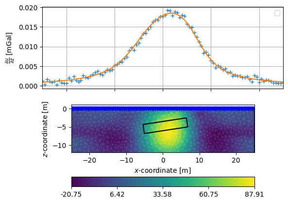
Visualization

For showing the model, we again plot model response and model.

fig, ax = pg.plt.subplots(ncols=1, nrows=2, sharex=True)
ax[0].plot(x, data, "+")
ax[0].plot(x, inv.response, "-")
ax[0].set_ylabel(r'$\frac{\partial u}{\partial z}$ [mGal]')
ax[0].grid()
ax[0].legend()

pg.show(mesh, rho, ax=ax[1], logScale=False)
pg.viewer.mpl.drawPLC(ax[1], rect, fillRegion=False)
ax[1].plot(x, x*0, 'bv')
ax[1].set_xlabel('$x$-coordinate [m]')
ax[1].set_ylabel('$z$-coordinate [m]')
ax[1].set_ylim((-12, 1))
ax[1].set_xlim((-25, 25))

(-25.0, 25.0)

References

• Li, Y. & Oldenburg, D. (1996): 3-D inversion of magnetic data. Geophysics 61(2), 394-408.

• Holstein, H., Sherratt, E.M., Reid, A.B.  (2007): Gravimagnetic field tensor gradiometry formulas for uniform polyhedra, SEG Ext. Abstr.