Note
Go to the end to download the full example code
Inversion with structural constraints#
Any inversion suffers from ambiguity and missing resolution at depth. Structural information can provide valuable information about geological boundaries in the subsurface. Such information can come from wave methods like seismics (Tanner et al. 2020), ground-penetrating radar (Doetsch et al. 2012, Jiang et al. 2020) or even piece-wise from boreholes (Wunderlich et al. 2018). This can be done in both 2D (Jiang et al. 2020) using lines or in 3D using facets (Doetsch et al. 2012).
We demonstrate on a very simple example from a bedrock detection how a structural interface from a seismic refraction can lead to models that are far easier to interpret.
# We import the numpy and matplotlib
import numpy as np
# Next we import pyGIMLi and the ERT and mesh tools modules
import pygimli as pg
import pygimli.meshtools as mt
from pygimli.physics import ert
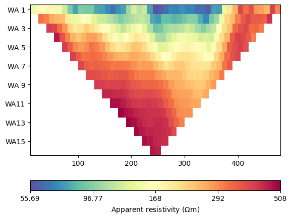
First we load the data and the interface
sphinx_gallery_thumbnail_number = 4
data = pg.getExampleData("ert/struct.dat")
xz = pg.getExampleData("ert/struct.txt")
ert.show(data)
(<Axes: >, <matplotlib.colorbar.Colorbar object at 0x7fe6e960b7c0>)
We estimate an error and do a normal inversion using the ERT manager. As we expect more or less layered structures, we choose a vertical weighting factor for the regularization of 0.5.
data.estimateError()
mgr = ert.Manager(data)
mgr.invert(paraDepth=150, zWeight=0.5, verbose=True)
fop: <pygimli.physics.ert.ertModelling.ERTModelling object at 0x7fe6e7c3a570>
Data transformation: <pygimli.core._pygimli_.RTransLogLU object at 0x7fe70971ef20>
Model transformation (cumulative):
         0 <pygimli.core._pygimli_.RTransLogLU object at 0x7fe6e955ea40>
min/max (data): 55.69/508
min/max (error): 3%/3%
min/max (start model): 254/254
--------------------------------------------------------------------------------
inv.iter 0 ... chi² =  343.06
--------------------------------------------------------------------------------
inv.iter 1 ... chi² =    9.41 (dPhi = 96.93%) lam: 20.0
--------------------------------------------------------------------------------
inv.iter 2 ... chi² =    7.32 (dPhi = 21.07%) lam: 20.0
--------------------------------------------------------------------------------
inv.iter 3 ... chi² =    6.16 (dPhi = 14.83%) lam: 20.0
--------------------------------------------------------------------------------
inv.iter 4 ... chi² =    5.10 (dPhi = 15.49%) lam: 20.0
--------------------------------------------------------------------------------
inv.iter 5 ... chi² =    3.27 (dPhi = 30.19%) lam: 20.0
--------------------------------------------------------------------------------
inv.iter 6 ... chi² =    0.42 (dPhi = 66.64%) lam: 20.0


################################################################################
#                  Abort criterion reached: chi² <= 1 (0.42)                   #
################################################################################

803 [61.641458462401,...,1465.6665066790185]
We plot the inversion result using a defined color scale. Additionally, we plot the measured line on top of it and see that generally there is a change from conductive overburden to resistive bedrock.
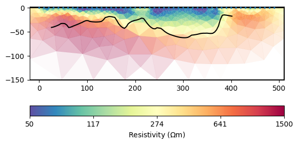
[<matplotlib.lines.Line2D object at 0x7fe6ea5ef2e0>]
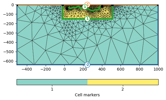
We now want to include this line into the inversion mesh. Therefore we generate the geometry of the inversion, a polygone from the line and merge both objects before we send it to the mesh generation.
plc = mt.createParaMeshPLC(data, paraDepth=150, boundary=1)
line = mt.createPolygon(xz, marker=1)
plc += line
mesh = mt.createMesh(plc, quality=34.3)
pg.show(mesh, markers=True, showMesh=True)
(<Axes: >, <matplotlib.colorbar.Colorbar object at 0x7fe735ab3580>)
We see the outer boundaries have markers of -1 (homogeneous Neumann, no-flow) and -2 (mixed) important to define the boundary conditions of the forward problem. The interface between the inversion domain (yellow) and the outer region (blue) and the added interface are >0 and do not affect the forward. We now use the generated mesh in a new ERT manager by setting it.
fop: <pygimli.physics.ert.ertModelling.ERTModelling object at 0x7fe6e7d20cc0>
Data transformation: <pygimli.core._pygimli_.RTransLogLU object at 0x7fe6eae1c360>
Model transformation: <pygimli.core._pygimli_.RTransLog object at 0x7fe6e853a6b0>
min/max (data): 55.69/508
min/max (error): 3%/3%
min/max (start model): 254/254
--------------------------------------------------------------------------------
inv.iter 0 ... chi² =  343.06
--------------------------------------------------------------------------------
inv.iter 1 ... chi² =    9.96 (dPhi = 96.63%) lam: 20.0
--------------------------------------------------------------------------------
inv.iter 2 ... chi² =    7.87 (dPhi = 19.95%) lam: 20.0
--------------------------------------------------------------------------------
inv.iter 3 ... chi² =    5.80 (dPhi = 23.98%) lam: 20.0
--------------------------------------------------------------------------------
inv.iter 4 ... chi² =    2.16 (dPhi = 50.36%) lam: 20.0
--------------------------------------------------------------------------------
inv.iter 5 ... chi² =    0.70 (dPhi = 42.69%) lam: 20.0


################################################################################
#                  Abort criterion reached: chi² <= 1 (0.70)                   #
################################################################################
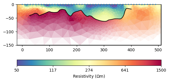
As a result, we see sharp resistivity jumps across the line in the center of the profile, i.e. the resistivity structure follows the given hints. At other positions like at the beginning of the profile, it does not show such strong contrasts indicating that the bedrock interface is probably more shallow and there is likely a weathered zone.
References Doetsch, J., Linde, N., Pessognelli, M., Green, A.G. & Günther, T. (2012): Constraining 3-D electrical resistance tomography with GPR data for improved aquifer characterization. Journal of Applied Geophysics 78, 68-76, doi:10.1016/j.jappgeo.2011.04.008. Wunderlich, T., Fischer, P., Wilken, D., Hadler, H., Erkul, E., Mecking, R., Günther, T., Heinzelmann, M., Vött, A. & Rabbel, W. (2018): Constraining Electric Resistivity Tomography by Direct Push Electric Conductivity logs and vibracores: An exemplary study of the Fiume Morto silted riverbed (Ostia Antica, Western Italy). Geophysics 83(3), B87-B103, doi:10.1190/geo2016-0660.1. Tanner, D.C., Buness, H., Igel, J., Günther, T., Gabriel, G., Skiba, P., Plenefisch, T., Gestermann, N. & Walter, T. (2020): Fault Detection. in: Tanner, C.D. & Brandes, C. (Eds.): Understanding Faults, 380p., Elsevier, 81-146, doi:10.1016/B978-0-12-815985-9.00003-5. Jiang, C., Igel, J., Dlugosch, R., Müller-Petke, M., Günther, T., Helms, J., Lang, J. & Winsemann (2020): Magnetic resonance tomography constrained by ground-penetrating radar for improved hydrogeophysical characterisation, Geophysics 85(6), JM13-JM26, doi:10.1190/geo2020-0052.1. Norooz, R., Olsson, P.-I., Dahlin, T., Günther, T. & Bernstone, C. (2021): A geoelectrical pre-study of Älvkarleby test embankment dam: 3D forward modelling and effects of structural constraints on the 3D inversion model of zoned embankment dams. J. Appl. Geophys. 191, 104355, doi:10.1016/j.jappgeo.2021.104355.
Total running time of the script: (0 minutes 32.707 seconds)