pygimli.physics.SIP

Spectral induced polarization (SIP) measurements and fittings.

Overview

Functions

ColeCole(f, R, m, tau, c[, a])
ColeColeEpsilon(f, e0, eInf, tau, alpha)
ColeColeRho(f, rho, m, tau, c[, a])
ColeColeRhoDouble(f, rho, m1, t1, c1, m2, t2, c2)
ColeColeSigma(f, sigma, m, tau, c[, a])
ColeDavidson(f, R, m, tau[, a])
drawAmplitudeSpectrum(ax, freq, amp[, ...])	Show amplitude spectrum (resistivity as a function of f).
drawPhaseSpectrum(ax, freq, phi[, ylabel, ...])	Show phase spectrum (-phi as a function of f).
load(fileName[, verbose])	Shortcut to load SIP spectral data.
modelColeColeEpsilon(f, e0, eInf, tau, alpha)	Original complex-valued permittivity formulation (Cole&Cole, 1941).
modelColeColeRho(f, rho, m, tau, c[, a])	Frequency-domain Cole-Cole impedance model after Pelton et al. (1978).
modelColeColeRhoDouble(f, rho, m1, t1, c1, ...)	Frequency-domain double Cole-Cole resistivity (impedance) model.
modelColeColeSigma(f, sigma, m, tau, c[, a])	Complex-valued conductivity (admittance) Cole-Cole model.
modelColeColeSigmaDouble(f, sigma, m1, t1, ...)	Complex-valued double added conductivity (admittance) model.
modelColeDavidson(f, R, m, tau[, a])	For backward compatibility.
showSpectrum(freq, amp, phi[, nrows, ylog, axs])	Show amplitude and phase spectra in two subplots.
tauRhoToTauSigma(tRho, m, c)	Convert \(\tau_{\rho}\) to \(\tau_{\sigma}\) Cole-Cole model.

Classes

ColeColeAbs(f[, verbose])	Cole-Cole model with EM term after Pelton et al. (1978).
ColeColeComplex(f[, verbose])	Cole-Cole model with EM term after Pelton et al. (1978).
ColeColeComplexSigma(f[, verbose])	Cole-Cole model with EM term after Pelton et al. (1978).
ColeColePhi(f[, verbose])	Cole-Cole model with EM term after Pelton et al. (1978).
DebyeComplex(fvec, tvec[, verbose])	Debye decomposition (smooth Debye relaxations) of complex data.
DebyePhi(fvec, tvec[, verbose])	Debye decomposition (smooth Debye relaxations) phase only.
DoubleColeColePhi(f[, verbose])	Double Cole-Cole model after Pelton et al. (1978).
PeltonPhiEM(f[, verbose])	Cole-Cole model with EM term after Pelton et al. (1978).
SIPSpectrum([filename, unify, onlydown, f, ...])	SIP spectrum data analysis.
SpectrumManager([fop])	Manager to work with spectra data.
SpectrumModelling([funct])	Modelling framework with an array of freqencies as data space.

Functions

pygimli.physics.SIP.ColeCole(f, R, m, tau, c, a=1)

pygimli.physics.SIP.ColeColeEpsilon(f, e0, eInf, tau, alpha)

pygimli.physics.SIP.ColeColeRho(f, rho, m, tau, c, a=1)

pygimli.physics.SIP.ColeColeRhoDouble(f, rho, m1, t1, c1, m2, t2, c2)

pygimli.physics.SIP.ColeColeSigma(f, sigma, m, tau, c, a=1)

pygimli.physics.SIP.ColeDavidson(f, R, m, tau, a=1)

pygimli.physics.SIP.drawAmplitudeSpectrum(ax, freq, amp, ylabel='$\\rho$ ($\\Omega$m)', grid=True, marker='+', ylog=True, **kwargs)

Show amplitude spectrum (resistivity as a function of f).

pygimli.physics.SIP.drawPhaseSpectrum(ax, freq, phi, ylabel='$-\\phi$ (mrad)', grid=True, marker='+', ylog=False, **kwargs)

Show phase spectrum (-phi as a function of f).

pygimli.physics.SIP.load(fileName, verbose=False, **kwargs)

Shortcut to load SIP spectral data.

Import Data and try to assume the file format.

Parameters:

fileName (str)

Returns:

freqs, amp, phi – Frequencies, amplitudes and phases phi in neg. radiant

Return type:

np.array

pygimli.physics.SIP.modelColeColeEpsilon(f, e0, eInf, tau, alpha)

Original complex-valued permittivity formulation (Cole&Cole, 1941).

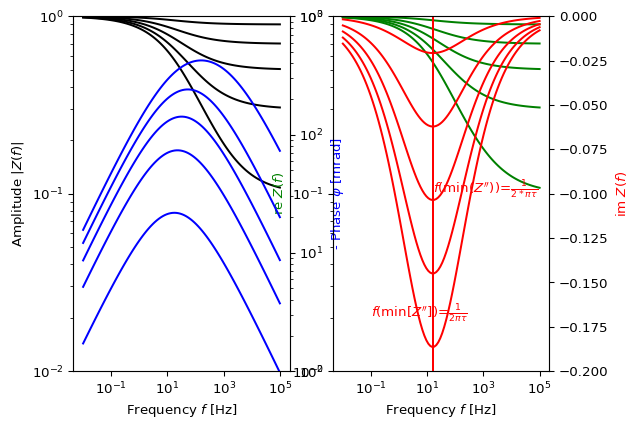
pygimli.physics.SIP.modelColeColeRho(f, rho, m, tau, c, a=1)

Frequency-domain Cole-Cole impedance model after Pelton et al. (1978).

Frequency-domain Cole-Cole impedance model after Pelton et al. (1978) [Pelton et al., 1978]

\[\begin{split}Z(\omega) & = \rho_0\left[1 - m \left(1 - \frac{1}{1+(\text{i}\omega\tau)^c}\right)\right] \\ \quad \text{with}\quad m & = \frac{1}{1+\frac{\rho_0}{\rho_1}} \quad \text{and}\quad \omega =2\pi f\end{split}\]

• \(Z(\omega)\) - Complex impedance per 1A current injection

• \(f\) - Frequency

• \(\rho_0\) – Background resistivity states the unblocked pore path

• \(\rho_1\) – Resistance of the solution in the blocked pore passages

• \(m\) – Chargeability after Seigel (1959) [Seigel, 1959] as being the ratio of voltage immediately after, to the voltage immediately before cessation of an infinitely long charging current.

• \(\tau\) – ‘Time constant’ relaxation time [s] for 1/e decay

• \(c\) - Rate of charge accumulation. Cole-Cole exponent typically [0.1 .. 0.6]

Examples

>>> import numpy as np
>>> import pygimli as pg
>>> from pygimli.physics.SIP import modelColeColeRho
>>> f = np.logspace(-2, 5, 100)
>>> m = np.linspace(0.1, 0.9, 5)
>>> tau = 0.01
>>> fImMin = 1/(tau*2*np.pi)
>>> fig, axs = pg.plt.subplots(1, 2)
>>> ax1 = axs[0]
>>> ax2 = axs[0].twinx()
>>> ax3 = axs[1]
>>> ax4 = axs[1].twinx()
>>> for i in range(len(m)):
...     Z = modelColeColeRho(f, rho=1, m=m[i], tau=tau, c=0.5)
...     _= ax1.loglog(f, np.abs(Z), color='black')
...     _= ax2.loglog(f, -np.angle(Z)*1000, color='b')
...     _= ax3.loglog(f, Z.real, color='g')
...     _= ax4.semilogx(f, Z.imag, color='r')
...     _= ax4.plot([fImMin, fImMin], [-0.2, 0.], color='r')
>>> _ = ax4.text(fImMin, -0.1, r"$f($min($Z''$))=$\frac{1}{2*\pi\tau}$", color='r')
>>> _ = ax4.text(0.1, -0.17, r"$f($min[$Z''$])=$\frac{1}{2\pi\tau}$", color='r')
>>> _ = ax1.set_ylabel('Amplitude $|Z(f)|$', color='black')
>>> _ = ax1.set_xlabel('Frequency $f$ [Hz]')
>>> _ = ax1.set_ylim(1e-2, 1)
>>> _ = ax2.set_ylabel(r'- Phase $\varphi$ [mrad]', color='b')
>>> _ = ax2.set_ylim(1, 1e3)
>>> _ = ax3.set_ylabel('re $Z(f)$', color='g')
>>> _ = ax4.set_ylabel('im $Z(f)$', color='r')
>>> _ = ax3.set_xlabel('Frequency $f$ [Hz]')
>>> _ = ax3.set_ylim(1e-2, 1)
>>> _ = ax4.set_ylim(-0.2, 0)
>>> pg.plt.show()

(png, pdf)

Examples using pygimli.physics.SIP.modelColeColeRho

Generating SIP signatures

Generating SIP signatures

Fitting SIP signatures

Fitting SIP signatures

pygimli.physics.SIP.modelColeColeRhoDouble(f, rho, m1, t1, c1, m2, t2, c2, a=1, mult=False)

Frequency-domain double Cole-Cole resistivity (impedance) model.

Frequency-domain Double Cole-Cole impedance model returns the sum of two Cole-Cole Models with a common amplitude. Z = rho * (Z1(Cole-Cole) + Z2(Cole-Cole))

pygimli.physics.SIP.modelColeColeSigma(f, sigma, m, tau, c, a=1)

Complex-valued conductivity (admittance) Cole-Cole model.

pygimli.physics.SIP.modelColeColeSigmaDouble(f, sigma, m1, t1, c1, m2, t2, c2, a=1, tauRho=True)

Complex-valued double added conductivity (admittance) model.

pygimli.physics.SIP.modelColeDavidson(f, R, m, tau, a=1)

For backward compatibility.

pygimli.physics.SIP.showSpectrum(freq, amp, phi, nrows=2, ylog=None, axs=None, **kwargs)

Show amplitude and phase spectra in two subplots.

pygimli.physics.SIP.tauRhoToTauSigma(tRho, m, c)

Convert \(\tau_{\rho}\) to \(\tau_{\sigma}\) Cole-Cole model.

\[\tau_{\sigma} = \tau_{\rho}/(1-m)^{\frac{1}{c}}\]

Examples

>>> import numpy as np
>>> import pygimli as pg
>>> from pygimli.physics.SIP import modelColeColeRho, modelColeColeSigma
>>> from pygimli.physics.SIP import tauRhoToTauSigma
>>> tr = 1.
>>> Z = modelColeColeRho(1e5, rho=10.0, m=0.5, tau=tr, c=0.5)
>>> ts = tauRhoToTauSigma(tr, m=0.5, c=0.5)
>>> S = modelColeColeSigma(1e5, sigma=0.1, m=0.5, tau=ts, c=0.5)
>>> abs(1.0/S - Z) < 1e-12
True
>>> float(np.angle(1.0/S / Z)) < 1e-12
True

Classes

class pygimli.physics.SIP.ColeColeAbs(f, verbose=False)

Bases: ModellingBaseMT__

Cole-Cole model with EM term after Pelton et al. (1978).

__init__((object)arg1[, (object)verbose=False]) → object :

C++ signature :

void* __init__(_object* [,bool=False])

__init__( (object)arg1, (object)dataContainer [, (object)verbose=False]) -> object :

C++ signature :

void* __init__(_object*,GIMLI::DataContainer {lvalue} [,bool=False])

__init__( (object)arg1, (object)mesh [, (object)verbose=False]) -> object :

C++ signature :

void* __init__(_object*,GIMLI::Mesh [,bool=False])

__init__( (object)arg1, (object)mesh, (object)dataContainer [, (object)verbose=False]) -> object :

C++ signature :

void* __init__(_object*,GIMLI::Mesh,GIMLI::DataContainer {lvalue} [,bool=False])

response(par)

Amplitude of the model.

class pygimli.physics.SIP.ColeColeComplex(f, verbose=False)

Bases: ModellingBaseMT__

Cole-Cole model with EM term after Pelton et al. (1978).

__init__((object)arg1[, (object)verbose=False]) → object :

C++ signature :

void* __init__(_object* [,bool=False])

__init__( (object)arg1, (object)dataContainer [, (object)verbose=False]) -> object :

C++ signature :

void* __init__(_object*,GIMLI::DataContainer {lvalue} [,bool=False])

__init__( (object)arg1, (object)mesh [, (object)verbose=False]) -> object :

C++ signature :

void* __init__(_object*,GIMLI::Mesh [,bool=False])

__init__( (object)arg1, (object)mesh, (object)dataContainer [, (object)verbose=False]) -> object :

C++ signature :

void* __init__(_object*,GIMLI::Mesh,GIMLI::DataContainer {lvalue} [,bool=False])

response(par)

Phase angle of the model.

class pygimli.physics.SIP.ColeColeComplexSigma(f, verbose=False)

Bases: ModellingBaseMT__

Cole-Cole model with EM term after Pelton et al. (1978).

__init__((object)arg1[, (object)verbose=False]) → object :

C++ signature :

void* __init__(_object* [,bool=False])

__init__( (object)arg1, (object)dataContainer [, (object)verbose=False]) -> object :

C++ signature :

void* __init__(_object*,GIMLI::DataContainer {lvalue} [,bool=False])

__init__( (object)arg1, (object)mesh [, (object)verbose=False]) -> object :

C++ signature :

void* __init__(_object*,GIMLI::Mesh [,bool=False])

__init__( (object)arg1, (object)mesh, (object)dataContainer [, (object)verbose=False]) -> object :

C++ signature :

void* __init__(_object*,GIMLI::Mesh,GIMLI::DataContainer {lvalue} [,bool=False])

response(par)

Phase angle of the model.

class pygimli.physics.SIP.ColeColePhi(f, verbose=False)

Bases: ModellingBaseMT__

Cole-Cole model with EM term after Pelton et al. (1978).

Modelling operator for the Frequency Domain Cole-Cole impedance model using pygimli.physics.SIP.modelColeColeRho after Pelton et al. (1978) [Pelton et al., 1978]

• \(\textbf{m} =\{ m, \tau, c\}\)

  Modelling parameter for the Cole-Cole model with \(\rho_0 = 1\)

• \(\textbf{d} =\{\varphi_i(f_i)\}\)

  Modelling response for all given frequencies as negative phase angles \(\varphi(f) = -tan^{-1}\frac{\text{Im}\,Z(f)}{\text{Re}\,Z(f)}\) and \(Z(f, \rho_0=1, m, \tau, c) =\) Cole-Cole impedance.

__init__(f, verbose=False)

Setup class by specifying the frequency.

response(par)

Phase angle of the model.

class pygimli.physics.SIP.DebyeComplex(fvec, tvec, verbose=False)

Bases: Modelling

Debye decomposition (smooth Debye relaxations) of complex data.

__init__(fvec, tvec, verbose=False)

Init with frequency and tau vector.

createJacobian(par)

Linear jacobian after Nordsiek&Weller (2008).

response(par)

amplitude/phase spectra as function of spectral chargeabilities.

class pygimli.physics.SIP.DebyePhi(fvec, tvec, verbose=False)

Bases: Modelling

Debye decomposition (smooth Debye relaxations) phase only.

__init__(fvec, tvec, verbose=False)

Init with frequency and tau vector.

response(par)

amplitude/phase spectra as function of spectral chargeabilities.

class pygimli.physics.SIP.DoubleColeColePhi(f, verbose=False)

Bases: ModellingBaseMT__

Double Cole-Cole model after Pelton et al. (1978).

Modelling operator for the Frequency Domain - phase only Cole-Cole impedance model using pygimli.physics.SIP.modelColeColeRho after Pelton et al. (1978) [Pelton et al., 1978]

• \(\textbf{m} =\{ m_1, \tau_1, c_1, m_2, \tau_2, c_2\}\)

  Modelling parameter for the Cole-Cole model with \(\rho_0 = 1\)

• \(\textbf{d} =\{\varphi_i(f_i)\}\)

  Modelling Response for all given frequencies as negative phase angles \(\varphi(f) = \varphi_1(Z_1(f))+\varphi_2(Z_2(f)) = -tan^{-1}\frac{\text{Im}\,(Z_1Z_2)}{\text{Re}\,(Z_1Z_2)}\) and \(Z_1(f, \rho_0=1, m_1, \tau_1, c_1)\) and \(Z_2(f, \rho_0=1, m_2, \tau_2, c_2)\) ColeCole impedances.

__init__(f, verbose=False)

Setup class by specifying the frequency.

response(par)

Phase angle of the model.

class pygimli.physics.SIP.PeltonPhiEM(f, verbose=False)

Bases: ModellingBaseMT__

Cole-Cole model with EM term after Pelton et al. (1978).

__init__((object)arg1[, (object)verbose=False]) → object :

C++ signature :

void* __init__(_object* [,bool=False])

__init__( (object)arg1, (object)dataContainer [, (object)verbose=False]) -> object :

C++ signature :

void* __init__(_object*,GIMLI::DataContainer {lvalue} [,bool=False])

__init__( (object)arg1, (object)mesh [, (object)verbose=False]) -> object :

C++ signature :

void* __init__(_object*,GIMLI::Mesh [,bool=False])

__init__( (object)arg1, (object)mesh, (object)dataContainer [, (object)verbose=False]) -> object :

C++ signature :

void* __init__(_object*,GIMLI::Mesh,GIMLI::DataContainer {lvalue} [,bool=False])

response(par)

Phase angle of the model.

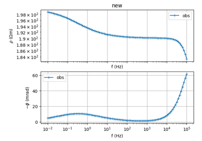
class pygimli.physics.SIP.SIPSpectrum(filename=None, unify=False, onlydown=True, f=None, amp=None, phi=None, k=1, sort=True, basename='new', **kwargs)

Bases: object

SIP spectrum data analysis.

__init__(filename=None, unify=False, onlydown=True, f=None, amp=None, phi=None, k=1, sort=True, basename='new', **kwargs)

Init SIP class with either filename to read or data vectors.

Examples

>>> #sip = SIPSpectrum('sipexample.txt', unify=True) # unique f values
>>> #sip = SIPSpectrum(f=f, amp=R, phi=phase, basename='new')

checkCRKK(useEps=False, use0=False, ax=None)

Check coupling removal (CR) by Kramers-Kronig (KK) relation.

cutF(fcut=1e+99, down=False)

Cut (delete) frequencies above a certain value fcut.

determineEpsilon(mode=0, sigmaR=None, sigmaI=None)

Retrieve frequency-independent epsilon for f->Inf.

Parameters:

• mode (int) –

  Operation mode:

  =0 - extrapolate using two highest frequencies (default) <0 - take last -n frequencies >0 - take n-th frequency

• sigmaR/sigmaI (float) – real and imaginary conductivity (if not given take data)

Returns:

er – relative permittivity (epsilon) value (dimensionless)

Return type:

float

epsilonR()

Calculate relative permittivity from imaginary conductivity.

fit2CCPhi(ePhi=0.001, lam=1000.0, mpar=(0, 0, 1), taupar1=(0, 1e-05, 1), taupar2=(0, 0.1, 1000), cpar=(0.5, 0, 1), verbose=False)

Fit two Cole-Cole terms (to phase only).

Parameters:

• ePhi (float) – absolute error of phase angle

• lam (float) – regularization parameter

• mpar (list[3]) – starting value, lower bound, upper bound for chargeability

• taupar2 (taupar1 /) – starting value, lower bound, upper bound for 2 time constants

• cpar2 (cpar1 /) – starting value, lower bound, upper bound for 2 relaxation exponents

fitCCEM(ePhi=0.001, lam=1000.0, remove=True, mpar=(0.2, 0, 1), taupar=(0.01, 1e-05, 100), cpar=(0.25, 0, 1), empar=(1e-07, 1e-09, 1e-05), verbose=False)

Fit a Cole-Cole term with additional EM term to phase.

Parameters:

• ePhi (float) – absolute error of phase angle

• lam (float) – regularization parameter

• remove (bool) – remove EM term from data

• mpar (list[3]) – inversion parameters (starting value, lower bound, upper bound) for Cole-Cole parameters (m, tau, c) and EM relaxation time (em)

• taupar (list[3]) – inversion parameters (starting value, lower bound, upper bound) for Cole-Cole parameters (m, tau, c) and EM relaxation time (em)

• cpar (list[3]) – inversion parameters (starting value, lower bound, upper bound) for Cole-Cole parameters (m, tau, c) and EM relaxation time (em)

• empar (list[3]) – inversion parameters (starting value, lower bound, upper bound) for Cole-Cole parameters (m, tau, c) and EM relaxation time (em)

fitCCPhi(ePhi=0.001, lam=1000.0, mpar=(0, 0, 1), taupar=(0, 1e-05, 100), cpar=(0.3, 0, 1), verbose=False)

Fit a Cole-Cole term (to phase only).

Parameters:

• ePhi (float) – absolute error of phase angle

• lam (float) – regularization parameter

• mpar (list[3]) – inversion parameters (starting value, lower bound, upper bound) for Cole-Cole parameters (m, tau, c) and EM relaxation time (em)

• taupar (list[3]) – inversion parameters (starting value, lower bound, upper bound) for Cole-Cole parameters (m, tau, c) and EM relaxation time (em)

• cpar (list[3]) – inversion parameters (starting value, lower bound, upper bound) for Cole-Cole parameters (m, tau, c) and EM relaxation time (em)

fitColeCole(useCond=False, **kwargs)

Fit a Cole-Cole model to the phase data.

Parameters:

• useCond (bool) – use conductivity form of Cole-Cole model instead of resistivity

• error (float [0.01]) – absolute phase error

• lam (float [1000]) – initial regularization parameter

• mpar (tuple/list (0, 0, 1)) – inversion parameters for chargeability: start, lower, upper bound

• taupar (tuple/list (1e-2, 1e-5, 100)) – inversion parameters for time constant: start, lower, upper bound

• cpar (tuple/list (0.25, 0, 1)) – inversion parameters for Cole exponent: start, lower, upper bound

fitDebyeModel(ePhi=0.001, lam=1000.0, lamFactor=0.8, tau=None, mint=None, maxt=None, nt=None, useComplex=True, showFit=False, verbose=False, **kwargs)

Fit a (smooth) continuous Debye model (Debye decomposition).

Parameters:

• ePhi (float) – absolute error of phase angle

• lam (float) – regularization parameter

• lamFactor (float) – regularization factor for subsequent iterations

• mint/maxt (float) – minimum/maximum tau values to use (else automatically from f)

• nt (int) – number of tau values (default number of frequencies * 2)

• new (bool) – new implementation (experimental)

• showFit (bool) – show fit

• cType (int) – constraint type (1/2=smoothness 1st/2nd order, 0=minimum norm)

• phi (iterable) – use phi instead of self.phi

fitDoubleColeCole(ePhi=0.001, eAmp=0.01, lam=1000.0, robust=False, verbose=True, useRho=True, useMult=False, aphi=True, mpar1=(0.2, 0, 1), mpar2=(0.2, 0, 1), tauRho=True, taupar1=(0.01, 1e-05, 100), taupar2=(0.0001, 1e-05, 100), cpar1=(0.5, 0, 1), cpar2=(0.5, 0, 1))

Fit double Cole-Cole term to complex resistivity or phase.

Parameters:

• ePhi (float [0.001]) – absolute error of phase angle in rad

• eAmp (float [0.01 = 1%]) – absolute error of phase angle

• lam (float) – regularization parameter

• robust (bool [False]) – use robustData (L1 norm on data side)

• useRho (bool [True]) – Cole-Cole defined for impedance/resistivity, otherwise conductivity

• useMult (bool [False]) – the two terms are combined as product (otherwise sum)

• tauRho (bool [False]) – in case of useRho=False the time constant is defined like for rho

• mpar1/2 (list[3]) – inversion parameters (starting value, lower bound, upper bound) for Cole-Cole parameters (m, tau, c)

• taupar1/2 (list[3]) – inversion parameters (starting value, lower bound, upper bound) for Cole-Cole parameters (m, tau, c)

• cpar1/2 (list[3]) – inversion parameters (starting value, lower bound, upper bound) for Cole-Cole parameters (m, tau, c)

getKK(use0=False)

Compute Kramers-Kronig impedance values (re->im and im->re).

getPhiKK(use0=False)

Compute phase from Kramers-Kronig quantities.

loadData(filename, **kwargs)

Import spectral data.

Import Data and try to assume the file format.

logMeanTau()

Mean logarithmic relaxation time (50% cumulative log curve).

omega()

Angular frequency.

realimag(cond=False)

Real and imaginary part of resistivity/conductivity (cond=True).

removeEpsilonEffect(er=None, mode=0)

Remove effect of (constant high-frequency) epsilon from sigma.

Parameters:

• er (float) – relative epsilon to correct for (else automatically determined)

• mode (int) – automatic epsilon determination mode (see determineEpsilon)

Returns:

er – determined permittivity (see determineEpsilon)

Return type:

float

saveFigures(name=None, ext='pdf')

Save all existing figures to files using file basename.

showAll(save=False, ax=None)

Plot spectrum, Cole-Cole fit and Debye distribution.

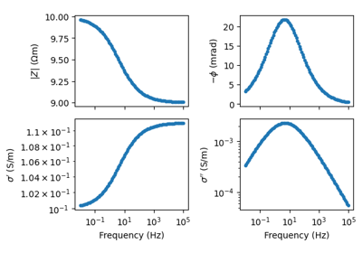
showData(reim=False, znorm=False, cond=False, nrows=2, ax=None, **kwargs)

Show amplitude and phase spectrum in two subplots.

Parameters:

• reim (bool) – show real/imaginary part instead of amplitude/phase

• znorm (bool (true forces reim)) – use normalized real/imag parts after Nordsiek&Weller (2008)

• (default=2) (nrows - use nrows subplots)

Returns:

fig, ax

Return type:

mpl.figure, mpl.axes array

showDataKK(use0=False)

Show data as real/imag subplots along with Kramers-Kronig curves.

showPhase(ax=None, **kwargs)

Plot phase spectrum (-phi over frequency).

showPolarPlot(cond=False)

Show data in a polar plot (imaginary vs. real parts).

sortData()

Sort data along increasing frequency (e.g. useful for KK).

totalChargeability()

Total chargeability (sum) from Debye curve.

unifyData(onlydown=False)

Unify data (only one value per frequency) by mean or selection.

zNorm()

Normalized real (difference) and imag. z [Nordsiek and Weller, 2008].

class pygimli.physics.SIP.SpectrumManager(fop=None, **kwargs)

Bases: MethodManager

Manager to work with spectra data.

__init__(fop=None, **kwargs)

Set up spectrum manager.

Parameters:

• fop (pg.Modelling operator, optional) – Forward operator. The default is None.

• **kwargs (TYPE) – passed to SpectrumManager.

createForwardOperator(**kwargs)

Create a Forward operator.

createInversionFramework(**kwargs)

Create inversion framework.

invert(data=None, f=None, **kwargs)

Invert the spectrum.

setData(freqs=None, amp=None, phi=None, eAmp=0.03, ePhi=0.001)

Set data for chosen sip model.

Parameters:

• freqs (iterable) – Array-like frequencies.

• amp (iterable) – Array-like amplitudes to work with.

• phi (iterable) – Array-like phase angles to work with.

• eAmp (float|iterable) – Relative error for amplitudes.

• ePhi (float|iterable) – Absolute error for phase angles.

setFunct(fop, **kwargs)

Set forward modelling function.

showResult()

Show resulting data.

simulate()

Make a simulation.

class pygimli.physics.SIP.SpectrumModelling(funct=None, **kwargs)

Bases: ParameterModelling

Modelling framework with an array of freqencies as data space.

Variables:

• params (dict)

• function (callable)

• complex (bool)

__init__(funct=None, **kwargs)

Initialize.

Parameters:

• func (function) – modelling function

• complex (bool) – complex function

• frequencies (iterable) – frequency vector

property complex

Return if spectrum is complex.

drawData(ax, data, err=None, **kwargs)

Draw data.

property freqs

Return frequency vector.

response(params)

Model response.

Parameters:

params (iterable) – model

Returns:

model response vector

Return type:

array_like