pygimli.physics.seismics

Full wave form seismics utilities and simulations

Overview

Functions

drawSeismogram(ax, mesh, u, dt[, ids, pos, i])	Extract and show time series from wave field
drawWiggle(ax, x, t[, xoffset, posColor, ...])	Draw signal in wiggle style into a given ax.
ricker(f, t[, t0])	Create Ricker wavelet.
solvePressureWave(mesh, velocities, times, ...)	Solve pressure wave equation.

Functions

pygimli.physics.seismics.drawSeismogram(ax, mesh, u, dt, ids=None, pos=None, i=None)

Extract and show time series from wave field

Parameters:

• ids (list) – List of node ids for the given mesh.

• pos (list) – List of positions for the given mesh. We will look for the nearest node.

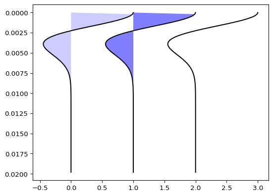
pygimli.physics.seismics.drawWiggle(ax, x, t, xoffset=0.0, posColor='red', negColor='blue', alpha=0.5, **kwargs)

Draw signal in wiggle style into a given ax.

Parameters:

• ax (matplotlib ax) – To plot into

• x (array [float]) – Signal.

• t (array) – Time base for x

• xoffset (float) – Move wiggle plot along x axis

• posColor (str) – Need to be convertible to matplotlib color. Fill positive areas with.

• negColor (str) – Need to be convertible to matplotlib color. Fill negative areas with.

• alpha (float) – Opacity for fill area.

• **kwargs (dict()) – Will be forwarded to matplotlib.axes.fill

Examples

>>> from pygimli.physics.seismics import ricker, drawWiggle
>>> import matplotlib.pyplot as plt
>>> import numpy as np
>>> t = np.arange(0, 0.02, 1./5000)
>>> r = ricker(t, 100., 1./100)
>>> fig = plt.figure()
>>> ax = fig.add_subplot(1,1,1)
>>> drawWiggle(ax, r, t, xoffset=0, posColor='red', negColor='blue',
...            alpha=0.2)
>>> drawWiggle(ax, r, t, xoffset=1)
>>> drawWiggle(ax, r, t, xoffset=2, posColor='black', negColor='white',
...            alpha=1.0)
>>> ax.invert_yaxis()
>>> plt.show()

(png, pdf)

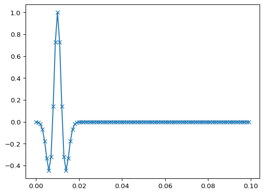
pygimli.physics.seismics.ricker(f, t, t0=0.0)

Create Ricker wavelet.

Create a Ricker wavelet with a desired frequency and signal length.

Parameters:

• f (float) – Frequency of the wavelet in Hz

• t (array [float]) – Time base definition

• t0 (float) – Offset time. Use 1/f to move the wavelet to start nearly from zero.

Returns:

y – Signal

Return type:

array_like

Examples

Create a 100 Hz Wavelet inside 1000 Hz sampled signal of length 0.1s.

>>> import matplotlib.pyplot as plt
>>> import numpy as np
>>> from pygimli.physics.seismics import ricker
>>> sampleFrequenz = 1000 #Hz
>>> t = np.arange(0, 0.1, 1./sampleFrequenz)
>>> r = ricker(100., t, 1./100)
>>> lines = plt.plot(t,r,'-x')
>>> plt.show()

(png, pdf)

pygimli.physics.seismics.solvePressureWave(mesh, velocities, times, sourcePos, uSource, verbose=False)

Solve pressure wave equation.

Solve pressure wave for a given source function

\[\begin{split}\frac{\partial^2 u}{\partial t^2} & = \diverg(a\grad u) + f\\ finalize equation\end{split}\]

Parameters:

• mesh (GIMLI::Mesh) – Mesh to solve on

• velocities (array) – velocities for each cell of the mesh

• time (array) – Time base definition

• sourcePos (RVector3) – Source position

• uSource (array) – u(t, sourcePos) source movement of length(times) Usually a Ricker wavelet of the desired seismic signal frequency.

Returns:

u – Return

Return type:

RMatrix

Examples

See TODO write example