pygimli.physics.ert#

Electrical Resistivity Tomography (ERT)

Direct-Current (DC) Resistivity and Induced Polarisation (IP)

This package contains tools, modelling operators, and managers for Electrical Resistivity Tomography (ERT) & Induced polarization (IP)

Main entry functions or classes: * simulate - synthetic (real or complex-valued) modelling * createData - generate data sets for synthetic modelling * ERTModelling - Modelling operator * ERTManager - data inversion and modelling for real resistivity * ERTIPManager - extension to IP (either frequency or time domain) * TimelapseERT - processing and inversion of timelapse ERT data * CrossholeERT - timelapse ERT in crosshole environments

Overview#

Functions

`coverageERT`	coverageDCtrans( (object)S, (object)dd, (object)mm) -> object :
`createData`(elecs[, schemeName])	Utility one-liner to create a BERT datafile
`createERTData`(args, *kwargs)
`createGeometricFactors`(args, *kwargs)
`createInversionMesh`(data, **kwargs)	Create default mesh for ERT inversion.
`drawERTData`(ax, data[, vals])	Plot ERT data as pseudosection matrix (position over separation).
`estimateError`(data[, relativeError, ...])	Estimate relative error based on relative and absolute parts.
`fitReciprocalErrorModel`(data[, nBins, show, rel])	Fit an error by statistical normal-reciprocal analysis.
`generateDataFromUniqueIndex`(ind[, data, nI])	Generate data container from unique index.
`generateDataPDF`(data[, filename])	Generate a multi-page pdf showing all data properties.
`geometricFactor`	geometricFactors( (object)data [, (object)dim=3 [, (object)forceFlatEarth=False]]) -> object :
`geometricFactors`(data [[, dim, forceFlatEarth])	Helper function to calculate configuration factors for a given DataContainerERT
`load`(fileName[, verbose])	Shortcut to load ERT data.
`reciprocalIndices`(data[, onlyOnce])	Return indices for reciprocal data.
`reciprocalProcessing`(data[, rel, maxrec, maxerr])	Reciprocal data analysis and error estimation.
`show`(data[, vals])	Plot ERT data as pseudosection matrix (position over separation).
`showData`(data[, vals])	Plot ERT data as pseudosection matrix (position over separation).
`showERTData`(data[, vals])	Plot ERT data as pseudosection matrix (position over separation).
`simulate`(mesh, scheme, res, **kwargs)	Simulate an ERT measurement.
`uniqueERTIndex`(data[, nI, reverse, unify])	Generate unique index from sensor indices A/B/M/N for matching

Classes

`CrossholeERT`([filename])	Class for crosshole ERT data manipulation.
`DataContainer`	alias of `DataContainerERT`
`ERTIPManager`(args, *kwargs)	Method manager for ERT including induced polarization (IP).
`ERTManager`([data])	ERT Manager.
`ERTModelling`([sr, verbose])	Forward operator for Electrical Resistivity Tomography.
`ERTModellingReference`(**kwargs)	Reference implementation for 2.5D Electrical Resistivity Tomography.
`Manager`	alias of `ERTManager`
`Modelling`	alias of `ERTModelling`
`TimelapseERT`([filename])	Class for crosshole ERT data manipulation.
`VESManager`(**kwargs)	Vertical electrical sounding (VES) manager class.
`VESModelling`([ab2, mn2])	Vertical Electrical Sounding (VES) forward operator.

Functions#

pygimli.physics.ert.coverageERT()#

coverageDCtrans( (object)S, (object)dd, (object)mm) -> object :

C++ signature :
GIMLI::Vector<double> coverageDCtrans(GIMLI::MatrixBase,GIMLI::Vector<double>,GIMLI::Vector<double>)

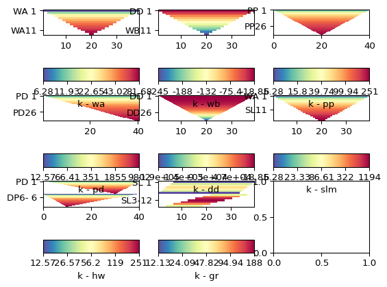
pygimli.physics.ert.createData(elecs, schemeName='none', **kwargs)[source]#

Utility one-liner to create a BERT datafile

Parameters:

elecs (int | list[pos] | array(x)) – Number of electrodes or electrode positions or x-positions
schemeName (str ['none']) – Name of the configuration. If you provide an unknown scheme name, all known schemes [‘wa’, ‘wb’, ‘pp’, ‘pd’, ‘dd’, ‘slm’, ‘hw’, ‘gr’] listed.
**kwargs –
Arguments that will be forwarded to the scheme generator.
- inversebool
  interchange AB MN with MN AB
- reciprocitybool
  interchange AB MN with BA NM
- addInversebool
  add additional inverse measurements
- spacingfloat [1]
  electrode spacing in meters
- closedbool
  Close the chain. Measure from the end of the array to the first electrode.

Returns:

data

Return type:

DataContainerERT

Examples

>>> import matplotlib.pyplot as plt
>>> from pygimli.physics import ert
>>>
>>> schemes = ['wa', 'wb', 'pp', 'pd', 'dd', 'slm', 'hw', 'gr']
>>> fig, ax = plt.subplots(3,3)
>>>
>>> for i, schemeName in enumerate(schemes):
...     s = ert.createData(elecs=41, schemeName=schemeName)
...     k = ert.geometricFactors(s)
...     _ = ert.show(s, vals=k, ax=ax.flat[i], label='k - ' + schemeName)
>>>
>>> plt.show()

(png, pdf)

Examples using pygimli.physics.ert.createData

2D ERT modelling and inversion

2D FEM modelling on two-layer example

Timelapse ERT

Complex-valued electrical modelling

Naive complex-valued electrical inversion

Synthetic TDIP modelling and inversion

Hydrogeophysical modelling

Petrophysical joint inversion

pygimli.physics.ert.createERTData(*args, **kwargs)#

pygimli.physics.ert.createGeometricFactors(*args, **kwargs)#

Examples using pygimli.physics.ert.createGeometricFactors

ERT field data with topography

Four-point sensitivities

ERT inversion of data measured on a standing tree

Naive complex-valued electrical inversion

pygimli.physics.ert.createInversionMesh(data, **kwargs)[source]#

Create default mesh for ERT inversion.

Parameters:: data (GIMLI::DataContainerERT) – Data Container needs at least sensors to define the geometry of the mesh.

:param Forwarded to pygimli.meshtools.createParaMesh:

Returns:: mesh – Inversion mesh with default marker (1 for background, 2 parametric domain)
Return type:: GIMLI::Mesh

pygimli.physics.ert.drawERTData(ax, data, vals=None, **kwargs)[source]#

Plot ERT data as pseudosection matrix (position over separation).

Parameters:

data (DataContainerERT) – data container with sensorPositions and a/b/m/n fields
vals (iterable of data.size() [data['rhoa']]) – vector containing the vals to show
ax (mpl.axis) – axis to plot, if not given a new figure is created
cMin/cMax (float) – minimum/maximum color vals
logScale (bool) – logarithmic colour scale [min(A)>0]
label (string) – colorbar label
**kwargs –
- dxfloat
  x-width of individual rectangles
- indinteger iterable or IVector
  indices to limit display
- circularbool
  Plot in polar coordinates when plotting via patchValMap

Returns:

ax – The used Axes
cbar – The used Colorbar or None

pygimli.physics.ert.estimateError(data, relativeError=0.03, absoluteUError=None, absoluteError=0, absoluteCurrent=0.1)[source]#

Estimate relative error based on relative and absolute parts.

Parameters:

relativeError (float [0.03]) – relative error level in %/100 for u, R or rhoa
absoluteUError (float [None]) – Absolute potential error in V. Needs ‘u’ values in data. Otherwise calculate them from ‘rhoa’, ‘k’ and absoluteCurrent if no ‘i’ given.
absoluteError (float [0.0]) – Absolute data error in Ohm m. Needs ‘R’ or ‘rhoa’ values.
absoluteCurrent (float [0.1]) – Current level in A for reconstruction for absolute potential V

Returns:

error

Return type:

Array

Examples using pygimli.physics.ert.estimateError

ERT field data with topography

3D surface ERT inversion

Region-wise regularization

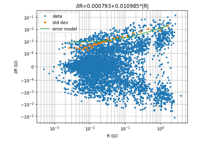
pygimli.physics.ert.fitReciprocalErrorModel(data, nBins=None, show=False, rel=False)[source]#

Fit an error by statistical normal-reciprocal analysis.

Identify normal reciprocal pairs and fit error model to it

Parameters:

data (pg.DataContainerERT) – input data
nBins (int) – number of bins to subdivide data (4 < data.size()//30 < 30)
rel (bool [False]) – fit relative instead of absolute errors
show (bool [False]) – generate plot of reciprocals, mean/std bins and error model

Returns:

ab – indices of a+b*R (rel=False) or a+b/R (rec=True)

Return type:

[float, float]

Examples using pygimli.physics.ert.fitReciprocalErrorModel

Reciprocal data analysis of field ERT data

pygimli.physics.ert.generateDataFromUniqueIndex(ind, data=None, nI=None)[source]#: Generate data container from unique index.

pygimli.physics.ert.generateDataPDF(data, filename='data.pdf')[source]#: Generate a multi-page pdf showing all data properties.

pygimli.physics.ert.geometricFactor()#

geometricFactors( (object)data [, (object)dim=3 [, (object)forceFlatEarth=False]]) -> object :

Helper function to calculate configuration factors for a given DataContainerERT

C++ signature :: GIMLI::Vector<double> geometricFactors(GIMLI::DataContainerERT [,int=3 [,bool=False]])

pygimli.physics.ert.geometricFactors((object)data[, (object)dim=3[, (object)forceFlatEarth=False]]) → object :#

Helper function to calculate configuration factors for a given DataContainerERT

C++ signature :: GIMLI::Vector<double> geometricFactors(GIMLI::DataContainerERT [,int=3 [,bool=False]])

Examples using pygimli.physics.ert.geometricFactors

2D crosshole ERT inversion

3D surface ERT inversion

3D crosshole ERT inversion

Region-wise regularization

pygimli.physics.ert.load(fileName, verbose=False, **kwargs)[source]#

Shortcut to load ERT data.

Import Data and try to assume the file format. Additionally to unified data format we support the wide-spread res2dinv format as well as ASCII column files generated by the processing software of various instruments (ABEM LS, Syscal Pro, Resecs, ?)

If this fails, install pybert and use its auto importer pybert.importData.

Parameters:: fileName (str) –
Returns:: data
Return type:: pg.DataContainer

pygimli.physics.ert.reciprocalIndices(data, onlyOnce=False)[source]#

Return indices for reciprocal data.

Parameters: data : DataContainerERT

data containing reciprocal data

onlyOncebool [False]: return every pair only once

Returns:: iN, iR – indices into the data container for normal and reciprocals
Return type:: np.array(dtype=int)

Examples using pygimli.physics.ert.reciprocalIndices

Reciprocal data analysis of field ERT data

pygimli.physics.ert.reciprocalProcessing(data, rel=True, maxrec=0.2, maxerr=0.2)[source]#

Reciprocal data analysis and error estimation.

Carry out workflow for reciprocal * identify normal reciprocal pairs * fit error model to it * estimate error for all measurements * remove one of the pairs (and duplicates) by averaging * filter the data for maximum reciprocity and error

Parameters:

out (pg.DataContainerERT) – input data container with possible
rel (bool) – base analysis on relative instead of absolute errors
maxrec (float [0.2]) – maximum reciprocity allowed in data
maxerr (float [0.2]) – maximum error estimate

Returns:

out – filtered data container with pairs removed/averaged

Return type:

pg.DataContainerERT

Examples using pygimli.physics.ert.reciprocalProcessing

Reciprocal data analysis of field ERT data

pygimli.physics.ert.show(data, vals=None, **kwargs)#

Plot ERT data as pseudosection matrix (position over separation).

Creates figure, axis and draw a pseudosection.

Parameters:

data (BERT::DataContainerERT) –
**kwargs –
- valsarray[nData] | str
  Values to be plotted. Default is data[‘rhoa’]. Can be array or string whose data field is extracted.
- axesmatplotlib.axes
  Axes to plot into. By default (None), a new figure with a single Axes is created.
- x and ystr | list(str)
  forces using matrix plot (drawDataContainerAsMatrix) x, y define the electrode number on x and y axis can be strings (“a”, “m”, “mid”, “sep”) or lists of them [“a”, “m”]
- stylestr
  predefined styles for choosing x and y arguments (x/y overrides) - “ab-mn” (default): any combination of current/potential electrodes - “a-m” : only a and m electrode (for unique dipole spacings like DD) - “a-mn” : a and combination of mn electrode (PD with different MN) - “ab-m” : a and combination of mn electrode - “sepa-m” : current dipole length with a and m (multi-gradient) - “a-sepm” : a and potential dipole length with m
- switchxybool
  exchange x and y axes before plotting

Returns:

ax (matplotlib.axes) – axis containing the plots
cb (matplotlib.colorbar) – colorbar instance

Examples using pygimli.physics.ert.show

2D ERT modelling and inversion

ERT field data with topography

ERT inversion of data measured on a standing tree

Timelapse ERT

Inversion with structural constraints

Incorporating prior data into ERT inversion

pygimli.physics.ert.showData(data, vals=None, **kwargs)#

Plot ERT data as pseudosection matrix (position over separation).

Creates figure, axis and draw a pseudosection.

Parameters:

data (BERT::DataContainerERT) –
**kwargs –
- valsarray[nData] | str
  Values to be plotted. Default is data[‘rhoa’]. Can be array or string whose data field is extracted.
- axesmatplotlib.axes
  Axes to plot into. By default (None), a new figure with a single Axes is created.
- x and ystr | list(str)
  forces using matrix plot (drawDataContainerAsMatrix) x, y define the electrode number on x and y axis can be strings (“a”, “m”, “mid”, “sep”) or lists of them [“a”, “m”]
- stylestr
  predefined styles for choosing x and y arguments (x/y overrides) - “ab-mn” (default): any combination of current/potential electrodes - “a-m” : only a and m electrode (for unique dipole spacings like DD) - “a-mn” : a and combination of mn electrode (PD with different MN) - “ab-m” : a and combination of mn electrode - “sepa-m” : current dipole length with a and m (multi-gradient) - “a-sepm” : a and potential dipole length with m
- switchxybool
  exchange x and y axes before plotting

Returns:

ax (matplotlib.axes) – axis containing the plots
cb (matplotlib.colorbar) – colorbar instance

Examples using pygimli.physics.ert.showData

ERT field data with topography

Petrophysical joint inversion

pygimli.physics.ert.showERTData(data, vals=None, **kwargs)[source]#

Plot ERT data as pseudosection matrix (position over separation).

Creates figure, axis and draw a pseudosection.

Parameters:

data (BERT::DataContainerERT) –
**kwargs –
- valsarray[nData] | str
  Values to be plotted. Default is data[‘rhoa’]. Can be array or string whose data field is extracted.
- axesmatplotlib.axes
  Axes to plot into. By default (None), a new figure with a single Axes is created.
- x and ystr | list(str)
  forces using matrix plot (drawDataContainerAsMatrix) x, y define the electrode number on x and y axis can be strings (“a”, “m”, “mid”, “sep”) or lists of them [“a”, “m”]
- stylestr
  predefined styles for choosing x and y arguments (x/y overrides) - “ab-mn” (default): any combination of current/potential electrodes - “a-m” : only a and m electrode (for unique dipole spacings like DD) - “a-mn” : a and combination of mn electrode (PD with different MN) - “ab-m” : a and combination of mn electrode - “sepa-m” : current dipole length with a and m (multi-gradient) - “a-sepm” : a and potential dipole length with m
- switchxybool
  exchange x and y axes before plotting

Returns:

ax (matplotlib.axes) – axis containing the plots
cb (matplotlib.colorbar) – colorbar instance

Examples using pygimli.physics.ert.showERTData

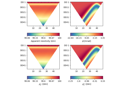
Complex-valued electrical modelling

Naive complex-valued electrical inversion

pygimli.physics.ert.simulate(mesh, scheme, res, **kwargs)[source]#

Simulate an ERT measurement.

Perform the forward task for a given mesh, resistivity distribution & measuring scheme and return data (apparent resistivity) or potentials.

For complex resistivity, the data contains an apparent phase or the returned potentials are complex.

The forward operator itself only calculates potential values for the electrodes in the given data scheme. To calculate apparent resistivities, geometric factors (k) are needed. If there are no values k in the DataContainerERT scheme, the function tries to calculate them, either analytically or numerically by using a p2-refined version of the given mesh.

Parameters:

mesh (GIMLI::Mesh) – 2D or 3D Mesh to calculate for.
res (float, array(mesh.cellCount()) | array(N, mesh.cellCount()) |) –
list Resistivity distribution for the given mesh cells can be: . float for homogeneous resistivity (e.g. 1.0) . single array of length mesh.cellCount() . matrix of N resistivity distributions of length mesh.cellCount() . resistivity map as [[regionMarker0, res0],

[regionMarker0, res1], …]
scheme (GIMLI::DataContainerERT) – Data measurement scheme.

Keyword Arguments:

verbose (bool[False]) – Be verbose. Will override class settings.
calcOnly (bool [False]) – Use fop.calculate instead of fop.response. Useful if you want to force the calculation of impedances for homogeneous models. No noise handling. Solution is put as token ‘u’ in the returned DataContainerERT.
noiseLevel (float [0.0]) – add normally distributed noise based on scheme[‘err’] or on noiseLevel if error>0 is not contained
noiseAbs (float [0.0]) – Absolute voltage error in V
returnArray (bool [False]) – Returns an array of apparent resistivities instead of a DataContainerERT
returnFields (bool [False]) – Returns a matrix of all potential values (per mesh nodes) for each injection electrodes.
sr (bool) – use secondary field (singularity removal)
seed (int) – numpy.random seed for repeatable noise in synthetic experiments
phiErr (float|iterable) – absolute phase error, if not given, data[‘iperr’] or noiseLevel is used
float|iterables (contactImpedances) – contact impedances for being used with CEM model

Returns:

DataContainerERT | array(data.size()) | array(N, data.size()) |
array(N, mesh.nodeCount()) – Data container with resulting apparent resistivity data[‘rhoa’] and errors (if noiseLevel or noiseAbs is set). Optionally return a Matrix of rhoa values (for returnArray==True forces noiseLevel=0). In case of complex-valued resistivity, phase values are contained in data[‘phia’] or returned as additionally returned array.

Examples

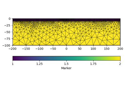
>>> from pygimli.physics import ert
>>> import pygimli as pg
>>> import pygimli.meshtools as mt
>>> world = mt.createWorld(start=[-50, 0], end=[50, -50],
...                        layers=[-1, -5], worldMarker=True)
>>> scheme = ert.createData(
...                     elecs=pg.utils.grange(start=-10, end=10, n=21),
...                     schemeName='dd')
>>> for pos in scheme.sensorPositions():
...     _= world.createNode(pos)
...     _= world.createNode(pos + [0.0, -0.1])
>>> mesh = mt.createMesh(world, quality=34)
>>> rhomap = [
...    [1, 100. + 0j],
...    [2, 50. + 0j],
...    [3, 10.+ 1j],
... ]
>>> data = ert.simulate(mesh, res=rhomap, scheme=scheme, verbose=True)

Examples using pygimli.physics.ert.simulate

2D ERT modelling and inversion

2D FEM modelling on two-layer example

Timelapse ERT

3D modelling in a closed geometry

Complex-valued electrical modelling

Naive complex-valued electrical inversion

Synthetic TDIP modelling and inversion

Petrophysical joint inversion

pygimli.physics.ert.uniqueERTIndex(data, nI=0, reverse=False, unify=True)[source]#

Generate unique index from sensor indices A/B/M/N for matching

Parameters:

data (DataContainerERT) – data container holding a b m n field registered as indices (int)
nI (int [0]) – index to generate (multiply), by default (0) sensorCount if two data files with different sensorCount are compared make sure to use the same nI for both
reverse (bool [False]) – exchange current (A, B) with potential (M, N) for reciprocal analysis
unify (bool [True]) – sort A/B and M/N so that bipole orientation does not matter

Classes#

class pygimli.physics.ert.CrossholeERT(filename=None, **kwargs)[source]#

Bases: TimelapseERT

Class for crosshole ERT data manipulation.

Note that this class is to be split into a hierarchy of classes for general timelapse data management, timelapse ERT and crosshole ERT. You can load data, filter them data in the temporal or measuring axis, plot data, run inversion and export data and result files.

__init__(filename=None, **kwargs)[source]#

Initialize class and possibly load data.

Parameters:

filename (str) – filename to load data, times, RHOA and ERR from
data (DataContainerERT) – The data with quadrupoles for all
times (np.array of datetime objects) – measuring times
DATA (2d np.array (data.size(), len(times))) – all apparent resistivities
ERR (2d np.array (data.size(), len(times))) – all apparent relative errors
bhmap (array) – map electrode numbers to borehole numbers
mesh (array) – mesh for inversion

createMesh(ibound=2, obound=10, quality=None, show=False, threeD=None, ref=0.25)[source]#

Create a 2D mesh around boreholes.

Parameters:

ibound (float) – inner boundary in m
ibound – outer boundary in m
quality (float) – triangle or tetgen quality
threeD (bool|None) – create 3D model (None-automatic)
ref (float) – electrode refinement in m

determineBHmap()[source]#: Auto-determine borehole map from xy positions.

extractSubset(nbh, plane=None, name=None)[source]#

Extract a subset (slice) by borehole number.

Returns a CrossholeERT instance with reduced boreholes

Parameters:

nbh (int|array) – borehole(s) to extract data from
name (str) – name to give the new instance
plane (bool [None]) – reduce to 2D (automatic if max. 2 boreholes are used)

load(filename, **kwargs)[source]#: Load or import data.

showData(v='rhoa', x='a', y='m', t=None, **kwargs)[source]#

Show data.

Show data as pseudosections (single-hole) or cross-plot (crosshole)

Parameters:

v (str|array ["rhoa]) – array or field to plot
x (str|array ["a", "m"]) – values to use for x and y axes
y (str|array ["a", "m"]) – values to use for x and y axes
t (int|str|datetime) – time to choose
kwargs (dict) – forwarded to ert.show or showDataContainerAsMatrix

pygimli.physics.ert.DataContainer#: alias of DataContainerERT

class pygimli.physics.ert.ERTIPManager(*args, **kwargs)[source]#

Bases: ERTManager

Method manager for ERT including induced polarization (IP).

This class should be use for any single IP data, which can be a single-frequency frequency-domain (FD) amplitude and phase, or a time-domain (TD) IP chargeability (one gate or an integral value).

__init__(*args, **kwargs)[source]#

Initialize DC part of it (parent class).

Parameters:: fd (bool) – Frequency-domain, otherwise time-domain

invert(*args, **kwargs)[source]#: Carry out DC and IP inversion.

invertFDIP(**kwargs)[source]#: IP inversion in frequency domain.

invertTDIP(ipdata='ip', **kwargs)[source]#: IP inversion in time domain.

saveResult(folder=None, *args, **kwargs)[source]#: Save all results in given or date-based folder.

showIPModel(**kwargs)[source]#: “Show IP model.

showResults(reskw={}, ipkw={}, **kwargs)[source]#

Show DC and IP results.

Parameters:

reskw (dict) – keyword arguments for showing resistivity image
ipkw (dict) – keyword arguments for showing IP image
**kwargs (dict) – keyword arguments for showing resistivity image

simulate(mesh, res, m, scheme=None, **kwargs)[source]#: .

class pygimli.physics.ert.ERTManager(data=None, **kwargs)[source]#

Bases: MeshMethodManager

ERT Manager.

Method Manager for Electrical Resistivity Tomography (ERT)

__init__(data=None, **kwargs)[source]#

Create ERT Manager instance.

Parameters:

data (GIMLI::DataContainerERT | str) – You can initialize the Manager with data or give them a dataset when calling the inversion.
useBert (*) – Use Bert forward operator instead of the reference implementation.
sr (*) – Calculate with singularity removal technique. Recommended but needs the primary potential. For flat earth cases the primary potential will be calculated analytical. For domains with topography the primary potential will be calculated numerical using a p2 refined mesh or you provide primary potentials with setPrimPot.

checkData(data=None)[source]#

Return data from container.

THINKABOUT: Data will be changed, or should the manager keep a copy?

checkErrors(err, dataVals)[source]#

Check (estimate) and return relative error.

By default we assume ‘err’ are relative values.

coverage()[source]#: Coverage vector considering the logarithmic transformation.

createForwardOperator(**kwargs)[source]#: Create and choose forward operator.

createMesh(data=None, **kwargs)[source]#

Create default inversion mesh.

Forwarded to pygimli.physics.ert.createInversionMesh

estimateError(data=None, **kwargs)[source]#

Estimate error composed of an absolute and a relative part.

Parameters:

absoluteError (float [0.001]) – Absolute data error in Ohm m. Need ‘rhoa’ values in data.
relativeError (float [0.03]) – relative error level in %/100
absoluteUError (float [0.001]) – Absolute potential error in V. Need ‘u’ values in data. Or calculate them from ‘rhoa’, ‘k’ and absoluteCurrent if no ‘i’ is given
absoluteCurrent (float [0.1]) – Current level in A for reconstruction for absolute potential V

Returns:

error

Return type:

Array

load(fileName)[source]#

Load ERT data.

Forwarded to pygimli.physics.ert.load

Parameters:: fileName (str) – Filename for the data.
Returns:: data
Return type:: GIMLI::DataContainerERT

saveResult(folder=None, size=(16, 10), **kwargs)[source]#

Save all results in the specified folder.

Saved items are:: Inverted profile Resistivity vector Coverage vector Standardized coverage vector Mesh (bms and vtk with results)

setSingularityRemoval(sr=True)[source]#: Turn singularity removal on or off.

showMisfit(errorWeighted=False, **kwargs)[source]#: Show relative or error-weighted data misfit.

showModel(model=None, ax=None, elecs=True, **kwargs)[source]#

Show the last inversion result.

Parameters:

model (iterable [None]) – Model vector to be drawn. Default is self.model from the last run
ax (mpl axes) – Axes object to draw into. Create a new if its not given.
elecs (bool) – Draw electrodes
**kwargs (dict) – arguments passed to pg.show (cMin, cMax, cMap, logScale)

Return type:

ax, cbar

simulate(*args, **kwargs)[source]#

Simulate an ERT measurement.

Perform the forward task for a given mesh, resistivity distribution & measuring scheme and return data (apparent resistivity) or potentials.

For complex resistivity, the apparent resistivities is complex as well.

Parameters:

mesh (GIMLI::Mesh) – 2D or 3D Mesh to calculate for.
res (float, array(mesh.cellCount()) | array(N, mesh.cellCount()) |) –
list Resistivity distribution for the given mesh cells can be: . float for homogeneous resistivity (e.g. 1.0) . single array of length mesh.cellCount() . matrix of N resistivity distributions of length mesh.cellCount() . resistivity map as [[regionMarker0, res0],

[regionMarker0, res1], …]
scheme (GIMLI::DataContainerERT) – Data measurement scheme.

Keyword Arguments:

verbose (bool[False]) – Be verbose. Will override class settings.
calcOnly (bool [False]) – Use fop.calculate instead of fop.response. Useful if you want to force the calculation of impedances for homogeneous models. No noise handling. Solution is put as token ‘u’ in the returned DataContainerERT.
noiseLevel (float [0.0]) – add normally distributed noise based on scheme[‘err’] or on noiseLevel if error>0 is not contained
noiseAbs (float [0.0]) – Absolute voltage error in V
returnArray (bool [False]) – Returns an array of apparent resistivities instead of a DataContainerERT
returnFields (bool [False]) – Returns a matrix of all potential values (per mesh nodes) for each injection electrodes.

Returns:

DataContainerERT | array(data.size()) | array(N, data.size()) |
array(N, mesh.nodeCount()) – Data container with resulting apparent resistivity data and errors (if noiseLevel or noiseAbs is set). Optional returns a Matrix of rhoa values (for returnArray==True forces noiseLevel=0). In case of a complex valued resistivity model, phase values are returned in the DataContainerERT (see example below), or as an additionally returned array.

Examples

# >>> from pygimli.physics import ert # >>> import pygimli as pg # >>> import pygimli.meshtools as mt # >>> world = mt.createWorld(start=[-50, 0], end=[50, -50], # … layers=[-1, -5], worldMarker=True) # >>> scheme = ert.createData( # … elecs=pg.utils.grange(start=-10, end=10, n=21), # … schemeName=’dd’) # >>> for pos in scheme.sensorPositions(): # … _= world.createNode(pos) # … _= world.createNode(pos + [0.0, -0.1]) # >>> mesh = mt.createMesh(world, quality=34) # >>> rhomap = [ # … [1, 100. + 0j], # … [2, 50. + 0j], # … [3, 10.+ 0j], # … ] # >>> data = ert.simulate(mesh, res=rhomap, scheme=scheme, verbose=1) # >>> rhoa = data.get(‘rhoa’).array() # >>> phia = data.get(‘phia’).array()

standardizedCoverage(threshold=0.01)[source]#: Return standardized coverage vector (0|1) using thresholding.

class pygimli.physics.ert.ERTModelling(sr=True, verbose=False)[source]#

Bases: ERTModellingBase

Forward operator for Electrical Resistivity Tomography.

Note

Convention for complex resistiviy inversion: We want to use logarithm transformation for the imaginary part of model so we need the startmodel to have positive imaginary parts. The sign is flipped back to physical correct assumption before we call the response function. The Jacobian is calculated with negative imaginary parts and will be a conjugated complex block matrix for further calulations.

__init__(sr=True, verbose=False)[source]#

Initialize.

Variables:

fop (pg.frameworks.Modelling) –
data (pg.DataContainer) –
modelTrans ([pg.trans.TransLog()]) –

Parameters:

**kwargs – fop : Modelling

createJacobian(mod)[source]#: Compute Jacobian matrix and store but not return.

createStartModel(dataVals)[source]#: Create Starting model for ERT inversion.

flipImagPart(v)[source]#: Flip imaginary port (convention).

response(mod)[source]#: Forward response (apparent resistivity).

setDataPost(data)[source]#: Set data (at a later stage).

setDefaultBackground()[source]#: Set the default background behaviour.

setMeshPost(mesh)[source]#: Set mesh (at a later stage).

setVerbose(v)[source]#: Set verbosity.

class pygimli.physics.ert.ERTModellingReference(**kwargs)[source]#

Bases: ERTModellingBase

Reference implementation for 2.5D Electrical Resistivity Tomography.

__init__(**kwargs)[source]#

Initialize.

Variables:

fop (pg.frameworks.Modelling) –
data (pg.DataContainer) –
modelTrans ([pg.trans.TransLog()]) –

Parameters:

**kwargs – fop : Modelling

calcGeometricFactor(data)[source]#: Calculate geometry factors for a given dataset.

createJacobian(model)[source]#: Create Jacobian matrix for model and store it in self.jacobian().

createRHS(mesh, elecs)[source]#: Create right-hand-side vector.

getIntegrationWeights(rMin, rMax)[source]#: TODO WRITEME.

mixedBC(boundary, userData)[source]#: Apply mixed boundary conditions.

pointSource(cell, f, userData)[source]#

Define function for the current source term.

$\delta(x-pos), \int f(x) \delta(x-pos)=f(pos)=N(pos)$: Right hand side entries will be shape functions(pos)

response(model)[source]#: Solve forward task and return apparent resistivity for self.mesh.

uAnalytical(p, sourcePos, k)[source]#: Calculate analytical potential for homogeneous halfspace.

For sigma = 1 [S m]

pygimli.physics.ert.Manager#: alias of ERTManager

pygimli.physics.ert.Modelling#: alias of ERTModelling

class pygimli.physics.ert.TimelapseERT(filename=None, **kwargs)[source]#

Bases: object

Class for crosshole ERT data manipulation.

__init__(filename=None, **kwargs)[source]#

Initialize class and possibly load data.

Parameters:

filename (str) – filename to load data, times, RHOA and ERR from
data (DataContainerERT) – The data with quadrupoles for all
times (np.array of datetime objects) – measuring times
DATA (2d np.array (data.size(), len(times))) – all apparent resistivities
ERR (2d np.array (data.size(), len(times))) – all apparent relative errors
bhmap (array) – map electrode numbers to borehole numbers
mesh (array) – mesh for inversion

chooseTime(t=None)[source]#

Return data for specific time.

Parameters:: t (int|str|datetime) –

createMesh(**kwargs)[source]#: Generate inversion mesh.

exportVTK(name=None, oneforall=False)[source]#: Generate output vtk(s) for postprocessing.

filter(tmin=0, tmax=None, t=None, select=None, kmax=None)[source]#

Filter data set temporally or data-wise.

Parameters:

tmin (int|str|datetime) – minimum and maximum times to keep
tmax (int|str|datetime) – minimum and maximum times to keep
t (int|str|datetime) – time to remove
select (list[int]) – times to select
kmax (float) – maximum geometric factor to allow

fitReciprocalErrorModel(**kwargs)[source]#

Fit all data by analysing normal/reciprocal data.

Parameters:

show (bool) – show temporal behaviour of absolute & relative errors
ert.fitReciprocalErrorModel) (kwargs passed on to) –

nBinsint
number of bins to subdivide data (4 < data.size()//30 < 30)

relbool [False]
fit relative instead of absolute errors

Returns:

p, a – relative (p) and absolute (a) errors for every time step

Return type:

array

fullInversion(scalef=1.0, **kwargs)[source]#: Full (4D) inversion.

generateDataPDF(**kwargs)[source]#

Generate a pdf with all data as timesteps in individual pages.

Iterates through times and calls showData into multi-page pdf

generateModelPDF(**kwargs)[source]#

Generate a multi-page pdf with the model results.

Parameters:: **kwargs (keyword arguments passed to pg.show()) –

generateRatioPDF(**kwargs)[source]#

Generate a multi-page pdf with the model results.

Parameters:

creep (bool [False]) – Use preceding time step as reference (default is baseline)
cMax (float [1/cMax]) – maximum of color scale
cMax – minimum of color scale
logScale (bool [True]) – logarithmic color scale
cMap (str ['bwr']) – colormap

invert(t=None, reg=None, regTL=None, **kwargs)[source]#

Run inversion for a specific timestep or all subsequently.

Parameter#

tint|datetime|str|array: time index, string or datetime object, or array of any of these
regdict: regularization options (setRegularization) for all inversions
regTLdict: regularization options for timesteps inversion only
**kwargsdict: keyword arguments passed to ERTManager.invert

load(filename)[source]#: Load or import data (or data files using *).

mask(rmin=0.1, rmax=1000000.0, emax=None)[source]#

Mask data (i.e. remove them from inversion).

Parameters:

rmin (float) – minimum and maximum apparent resistivity
rmax (float) – minimum and maximum apparent resistivity
emax (float) – maximum error

saveData(filename=None)[source]#: Save all data as datacontainer, times, rhoa and error arrays.

showAllModels(ncols=2, **kwargs)[source]#

Show all models as subplots.

Parameters:

ncols (int [2]) – number of columns
**kwargs (dict) – keyword arguments passed to pg.show

showData(v='rhoa', x='a', y='m', t=None, **kwargs)[source]#

Show data as pseudosections (single-hole) or cross-plot (crosshole)

Parameters:

v (str|array ["rhoa]) – array or field to plot
x (str|array ["a", "m"]) – values to use for x and y axes
y (str|array ["a", "m"]) – values to use for x and y axes
t (int|str|datetime) – time to choose
kwargs (dict) – forwarded to ert.show or showDataContainerAsMatrix

showFit(**kwargs)[source]#: Show data, model response and misfit.

showTimeline(ax=None, **kwargs)[source]#

Show data timeline.

Parameters:

ax (mpl.Axes|None) – matplotlib axes to plot (otherwise new)
a (int) – tokens to extract data from
b (int) – tokens to extract data from
m (int) – tokens to extract data from
n (int) – tokens to extract data from

timeIndex(t)[source]#

Return index of closest timestep in times to t.

Parameters:: t (int|str|datetime) – datetime object or string

class pygimli.physics.ert.VESManager(**kwargs)[source]#

Bases: MethodManager1d

Vertical electrical sounding (VES) manager class.

Examples

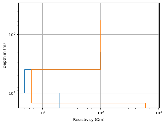
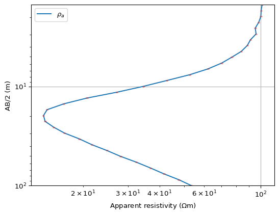
>>> import numpy as np
>>> import pygimli as pg
>>> from pygimli.physics import VESManager
>>> ab2 = np.logspace(np.log10(1.5), np.log10(100), 32)
>>> mn2 = 1.0
>>> # 3 layer with 100, 500 and 20 Ohmm
>>> # and layer thickness of 4, 6, 10 m
>>> # over a Halfspace of 800 Ohmm
>>> synthModel = pg.cat([4., 6., 10.], [100., 5., 20., 800.])
>>> ves = VESManager()
>>> ra, err = ves.simulate(synthModel, ab2=ab2, mn2=mn2, noiseLevel=0.01)
>>> ax = ves.showData(ra, error=err)
>>> model = ves.invert(ra, err, nLayers=4, showProgress=0, verbose=0)
>>> ax, _ = ves.showModel(synthModel)
>>> _ = ves.showResult(ax=ax)

../../_images/pygimli-physics-ert-2_00.png — (`png`, `pdf`)#

../../_images/pygimli-physics-ert-2_01.png — (`png`, `pdf`)#

__init__(**kwargs)[source]#

Initialize instance.

Parameters:: complex (bool) – Accept complex resistivities.
Variables:: complex (bool) – Accept complex resistivities.

property complex#: Return whether the computations are complex.

createForwardOperator(**kwargs)[source]#

Create Forward Operator.

Create Forward Operator based on complex attribute.

exportData(fileName, data=None, error=None)[source]#

Export data into simple ascii matrix.

Usefull?

invert(data=None, err=None, ab2=None, mn2=None, **kwargs)[source]#

Invert measured data.

Parameters:

data (iterable) – data vector
err (iterable) – error vector
ab2 (iterable) – AB/2 vector (otherwise taken from data)
mn2 (iterable) – MN/2 vector (otherwise taken from data)

Keyword Arguments:

**kwargs – Additional kwargs inherited from %(MethodManager1d.invert) and %(Inversion.run)

Returns:

model – inversion result

Return type:

pg.Vector

loadData(fileName, **kwargs)[source]#: Load simple data matrix.

preErrorCheck(err, dataVals=None)[source]#: Fct to be called before the validity check of the error values.

simulate(model, ab2=None, mn2=None, **kwargs)[source]#: Simulate measurement data.

class pygimli.physics.ert.VESModelling(ab2=None, mn2=None, **kwargs)[source]#

Bases: Block1DModelling

Vertical Electrical Sounding (VES) forward operator.

Variables:

ab2 – Half distance between the current electrodes A and B.
mn2 – Half distance between the potential electrodes M and N. Only used for input (feeding am etc.) or plotting.
am – Part of data basis. Distances between A and M electrodes. A is first current, M is first potential electrode.
bm – Part of data basis. Distances between B and M electrodes. B is second current, M is first potential electrode.
an – Part of data basis. Distances between A and N electrodes. A is first current, N is second potential electrode.
bn – Part of data basis. Distances between B and N electrodes. B is second current, N is second potential electrode.

__init__(ab2=None, mn2=None, **kwargs)[source]#

Initialize with distances.

Either with * all distances AM, AN, BM, BN using am/an/bm/bn * a dataContainerERT using data or dataContainerERT * AB/2 and (optionally) MN/2 distances using ab2/mn2

nLayersint [4]: Number of layers.

createStartModel(rhoa)[source]#: Create starting model.

drawData(ax, data, error=None, label=None, **kwargs)[source]#

Draw modeled apparent resistivity data.

Parameters:

ax (axes) – Matplotlib axes object to draw into.
data (iterable) – Apparent resistivity values to draw.
error (iterable [None]) – Adds an error bar if you have error values.
label (str ['$rho_a$']) – Set legend label for the amplitude.
ab2 (iterable) – Override ab2 that fits data size.
mn2 (iterable) – Override mn2 that fits data size.
plot (function name) – Matplotlib plot function, e.g., plot, loglog, semilogx or semilogy

drawModel(ax, model, **kwargs)[source]#: Draw model as 1D block model.

response(par)[source]#: Model response.

response_mt(par, i=0)[source]#: Multi-threading model response.

setDataSpace(ab2=None, mn2=None, am=None, bm=None, an=None, bn=None, **kwargs)[source]#

Set data basis, i.e., arrays for all am, an, bm, bn distances.

You can set either * AB/2 and (optionally) MN/2 spacings for a classical sounding, or * all distances AM, AN, BM, BN for arbitrary arrays :param ab2: AB/2 distances :type ab2: iterable :param mn2: MN/2 distance(s) :type mn2: iterable | float :param am: :type am: distances between current and potential electrodes :param an: :type an: distances between current and potential electrodes :param bm: :type bm: distances between current and potential electrodes :param bn: :type bn: distances between current and potential electrodes