Note

Go to the end to download the full example code

Region-wise regularization#

In this tutorial we like to demonstrate how to control the regularization of subsurface regions individually by using an ERT field case. The data is a 2d profile that was measured in 2005 on the bottom of a lake. The water body is of course influencing the fields and needs to be treated accordingly.

We first import pygimli and the modules for ERT and mesh building.

import matplotlib.pyplot as plt
import pygimli as pg
from pygimli.physics import ert
import pygimli.meshtools as mt

Data and geometry#

The data was measured across a shallow lake with the most electrodes being on the bottom of a lake. We used cables with 2m spaced takeouts.

data = pg.getExampleData("ert/lake.ohm")
print(data)

Data: Sensors: 48 data: 658, nonzero entries: ['a', 'b', 'err', 'i', 'm', 'n', 'r', 'u', 'valid']

The data consists of 658 data with current and voltage using 48 electrodes. We first have a look at the electrode positions measured by a stick.

plt.plot(pg.x(data), pg.z(data), "o-")
plt.grid()

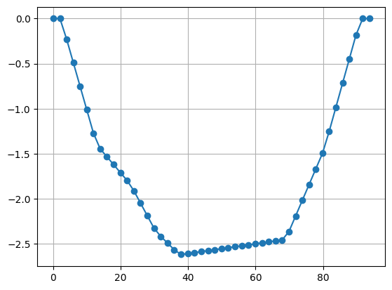
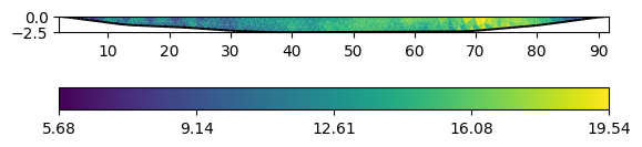
On both sides, two electrodes are on shore, but the others are on the bottom of a shallow lake with a maximum depth of 2.5m.

data["k"] = ert.geometricFactors(data)
data["rhoa"] = data["u"] / data["i"] * data["k"]
ax, cb = data.show()

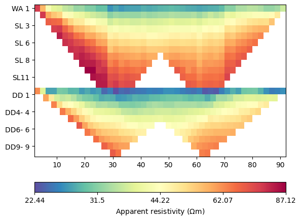
We combined Wenner-Schlumberger (top) and Wenner-beta (bottom) data. The lowest resistivities correspond with the water resistivity of 22.5 :math:`Omega`m.

The contained errors are measured standard devitations and should not be used for inversion. Instead, we estimate new errors using 2% and 100microVolts.

data["err"] = ert.estimateError(data, relativeError=0.02, absoluteUError=1e-4)
print(max(data["err"]))
# pg.show(data, data["err"]*100, label="error (%)");

0.02584795321637427

Building a mesh with the water body#

# We create a piece-wise linear complex (PLC) as for a case with topography
plc = mt.createParaMeshPLC(data, paraDepth=20, boundary=1)
ax, _ = pg.show(plc, markers=True)
for i, n in enumerate(plc.nodes()[:12]):
    ax.text(n.x(), n.y(), str(i))
    print(i, n.x(), n.y())

-4.0 0.0
-4.0 -20.0
97.7452 -20.0
97.7452 0.0
-97.7452 0.0
-97.7452 -113.7452
191.4904 0.0
191.4904 -113.7452
0.0 0.0
1.0 0.0
2.0 0.0
2.993365 -0.11499999999999999

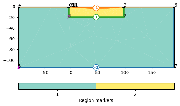
So node number 10 is the left one at the shore

for i in range(95, plc.nodeCount()):
    print(i, plc.node(i).x(), plc.node(i).y())

86.7804 -0.5833335
87.7715 -0.45
88.76255 -0.3166665
89.75359999999999 -0.183333
90.7494 -0.0916665
91.7452 0.0
92.7452 0.0
93.7452 0.0

and 100 the first on the other side. We connect nodes 10 and 100 by an edge

plc.createEdge(plc.node(10), plc.node(100), marker=-1)
plc.addRegionMarker([50, -0.1], marker=3)
ax, _ = pg.show(plc, markers=True)

As the lake bottom is not a surface boundary (-1) anymore, but an inside boundary, we set its marker >0 by iterating through all boundaries.

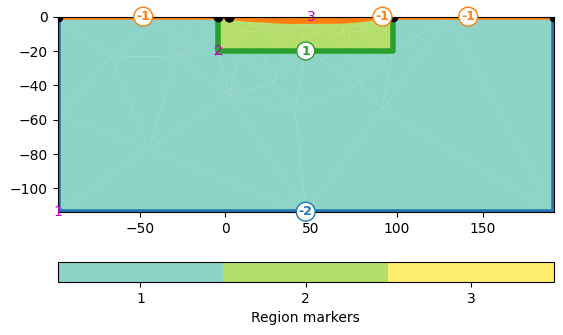
mesh = mt.createMesh(plc, quality=34.2)
for b in mesh.boundaries():
    if b.marker() == -1 and not b.outside():
        b.setMarker(2)

print(mesh)
ax, _ = pg.show(mesh, markers=True, showMesh=True)

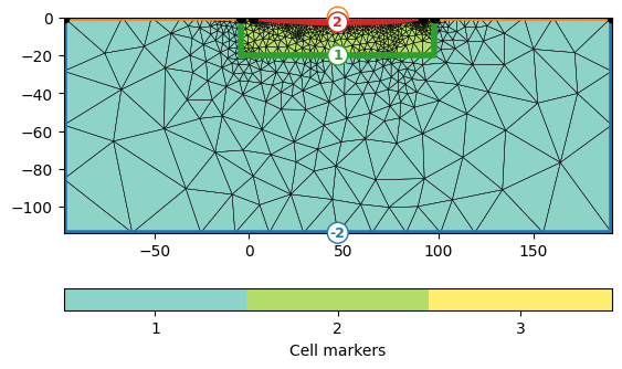
Mesh: Nodes: 1188 Cells: 2217 Boundaries: 3404

Inversion with the ERT manager#

mgr = ert.ERTManager(data, verbose=True)
mgr.setMesh(mesh)  # use this mesh for all subsequent runs
mgr.invert()
# mgr.invert(mesh=mesh) would only temporally use the mesh

fop: <pygimli.physics.ert.ertModelling.ERTModelling object at 0x7fe735330f90>
Data transformation: <pygimli.core._pygimli_.RTransLogLU object at 0x7fe735dc5800>
Model transformation: <pygimli.core._pygimli_.RTransLog object at 0x7fe6e9a0c360>
min/max (data): 22.44/87.12
min/max (error): 2%/2.58%
min/max (start model): 47.2/47.2
--------------------------------------------------------------------------------
inv.iter 0 ... chi² =  211.20
--------------------------------------------------------------------------------
inv.iter 1 ... chi² =   60.46 (dPhi = 71.32%) lam: 20.0
--------------------------------------------------------------------------------
inv.iter 2 ... chi² =   19.19 (dPhi = 67.98%) lam: 20.0
--------------------------------------------------------------------------------
inv.iter 3 ... chi² =    7.60 (dPhi = 59.42%) lam: 20.0
--------------------------------------------------------------------------------
inv.iter 4 ... chi² =    4.68 (dPhi = 37.43%) lam: 20.0
--------------------------------------------------------------------------------
inv.iter 5 ... chi² =    3.15 (dPhi = 31.27%) lam: 20.0
--------------------------------------------------------------------------------
inv.iter 6 ... chi² =    1.80 (dPhi = 39.61%) lam: 20.0
--------------------------------------------------------------------------------
inv.iter 7 ... chi² =    1.80 (dPhi = -0.28%) lam: 20.0
################################################################################
#                Abort criterion reached: dPhi = -0.28 (< 2.0%)                #
################################################################################

1751 [243.48637735106445,...,129.55314992715358]

The fit is obviously not perfect. So we have a look at data and model response.

ax = mgr.showFit()

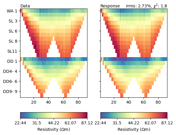
Both look very similar, but let us look at the misfit function in detail.

mgr.showMisfit(errorWeighted=True)

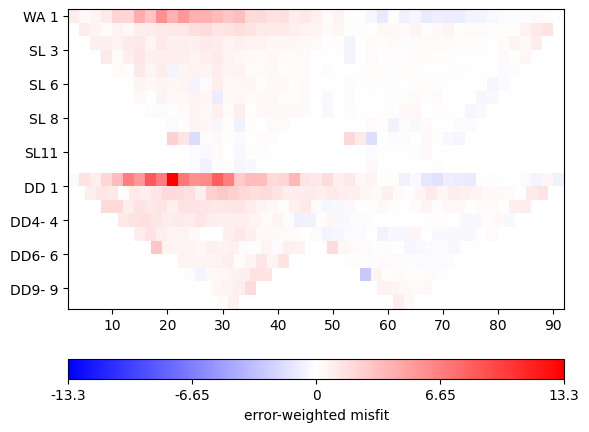
There is still systematics in the misfit. Ideally it should be a random distribution of Gaussian noise.

cov = pg.Vector(mgr.model.size(), 1.0)
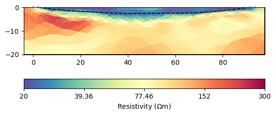
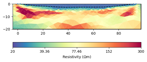
kw = dict(cMin=20, cMax=300, logScale=True, cMap="Spectral_r", coverage=cov)
ax, cb = mgr.showResult(**kw)

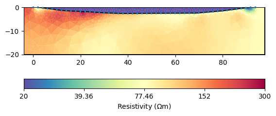
Apparently, the two regions are already decoupled from each other which makes sense. Let us look in detail at the water cells by extracting the water body. Note. The manager class performs a model value permutation to fit the parametric mesh cell. So if you want to relate model values to the input mesh, you need to use the unpermutated model values directly from the inversion framework instance: mgr.fw.model`

water = mesh.createSubMesh(mesh.cells(mesh.cellMarkers() == 3))
resWater = mgr.fw.model[len(mgr.model)-water.cellCount():]
ax, cb = pg.show(water, resWater)

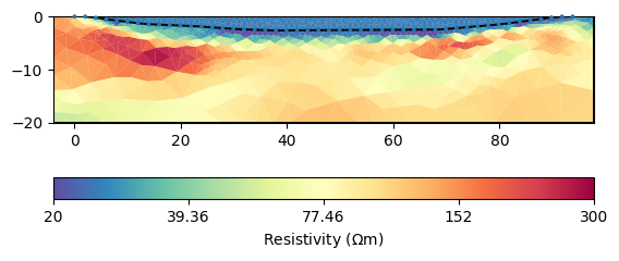
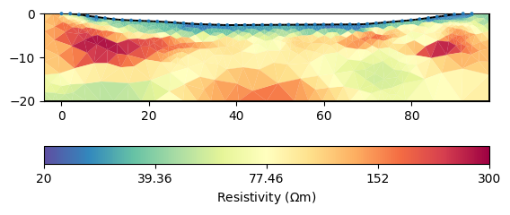
Apparently, all values are below the expected 22.5 :math:`Omega`m and some are implausibly low. Therefore we should try to limit them. Moreover, the subsurface structures do not look very “layered”, which is why we make the smoothness anisotropic.

mgr.inv.setRegularization(zWeight=0.1)
mgr.invert()
# mgr.invert(zWeight=0.1)  # only temporarily
ax, cb = mgr.showResult(**kw)

fop: <pygimli.physics.ert.ertModelling.ERTModelling object at 0x7fe735330f90>
Data transformation: <pygimli.core._pygimli_.RTransLogLU object at 0x7fe735dc5800>
Model transformation (cumulative):
         0 <pygimli.core._pygimli_.RTransLogLU object at 0x7fe6e8f9dea0>
         1 <pygimli.core._pygimli_.RTransLogLU object at 0x7fe6e8f9dea0>
min/max (data): 22.44/87.12
min/max (error): 2%/2.58%
min/max (start model): 47.2/47.2
--------------------------------------------------------------------------------
inv.iter 0 ... chi² =  211.20
--------------------------------------------------------------------------------
inv.iter 1 ... chi² =   54.09 (dPhi = 74.36%) lam: 20.0
--------------------------------------------------------------------------------
inv.iter 2 ... chi² =   19.93 (dPhi = 63.09%) lam: 20.0
--------------------------------------------------------------------------------
inv.iter 3 ... chi² =    5.53 (dPhi = 72.07%) lam: 20.0
--------------------------------------------------------------------------------
inv.iter 4 ... chi² =    2.41 (dPhi = 55.71%) lam: 20.0
--------------------------------------------------------------------------------
inv.iter 5 ... chi² =    0.74 (dPhi = 67.45%) lam: 20.0


################################################################################
#                  Abort criterion reached: chi² <= 1 (0.74)                   #
################################################################################

Region-specific regularization#

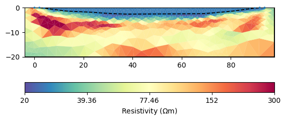
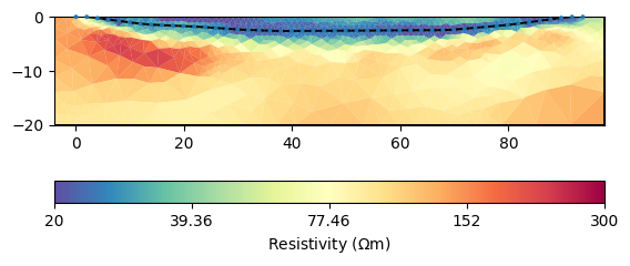
We first want to limit the resistivity of the water between some plausible bounds around our measurements.

mgr.inv.setRegularization(3, limits=[20, 25], trans="log")
mgr.invert()
ax, cb = mgr.showResult(**kw)

fop: <pygimli.physics.ert.ertModelling.ERTModelling object at 0x7fe735330f90>
Data transformation: <pygimli.core._pygimli_.RTransLogLU object at 0x7fe735dc5800>
Model transformation (cumulative):
         0 <pygimli.core._pygimli_.RTransLogLU object at 0x7fe6e8f9c6a0>
         1 <pygimli.core._pygimli_.RTransLogLU object at 0x7fe7089a7940>
min/max (data): 22.44/87.12
min/max (error): 2%/2.58%
min/max (start model): 47.2/47.2
--------------------------------------------------------------------------------
inv.iter 0 ... chi² =  211.20
--------------------------------------------------------------------------------
inv.iter 1 ... chi² =   65.55 (dPhi = 68.92%) lam: 20.0
--------------------------------------------------------------------------------
inv.iter 2 ... chi² =   24.23 (dPhi = 62.88%) lam: 20.0
--------------------------------------------------------------------------------
inv.iter 3 ... chi² =    3.31 (dPhi = 85.91%) lam: 20.0
--------------------------------------------------------------------------------
inv.iter 4 ... chi² =    0.46 (dPhi = 83.37%) lam: 20.0


################################################################################
#                  Abort criterion reached: chi² <= 1 (0.46)                   #
################################################################################

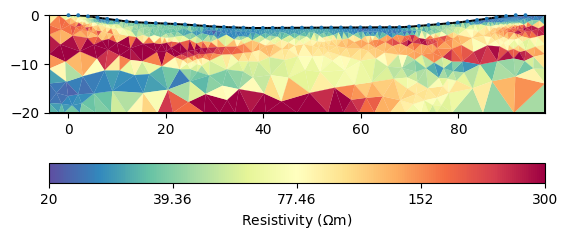
As a result of the log-log transform, we have a homogeneous body but below the lake bottom values below 20, maybe due to clay content or maybe as compensation of limiting the water resistivity too strong. We could limit the subsurface, too.

mgr.inv.setRegularization(2, limits=[20, 2000], trans="log")
mgr.invert()
ax, cb = mgr.showResult(**kw)

fop: <pygimli.physics.ert.ertModelling.ERTModelling object at 0x7fe735330f90>
Data transformation: <pygimli.core._pygimli_.RTransLogLU object at 0x7fe735dc5800>
Model transformation (cumulative):
         0 <pygimli.core._pygimli_.RTransLogLU object at 0x7fe6e8cafb20>
         1 <pygimli.core._pygimli_.RTransLogLU object at 0x7fe708affb80>
min/max (data): 22.44/87.12
min/max (error): 2%/2.58%
min/max (start model): 47.2/47.2
--------------------------------------------------------------------------------
inv.iter 0 ... chi² =  211.20
--------------------------------------------------------------------------------
inv.iter 1 ... chi² =   43.38 (dPhi = 79.21%) lam: 20.0
--------------------------------------------------------------------------------
inv.iter 2 ... chi² =   24.17 (dPhi = 43.41%) lam: 20.0
--------------------------------------------------------------------------------
inv.iter 3 ... chi² =    2.57 (dPhi = 87.85%) lam: 20.0
--------------------------------------------------------------------------------
inv.iter 4 ... chi² =    0.84 (dPhi = 59.98%) lam: 20.0


################################################################################
#                  Abort criterion reached: chi² <= 1 (0.84)                   #
################################################################################

Apparently, this makes it harder to fit the data accurately. So maybe an increased clay content can be responsible for resistivity below 20:math:`Omega`m in the mud.

Model reduction#

Another option is to treat the water body as a homogeneous body with only one unknown in the inversion.

mgr.inv.setRegularization(limits=[0, 0], trans="log")
mgr.inv.setRegularization(3, single=True)
mgr.invert()
ax, cb = mgr.showResult(**kw)

fop: <pygimli.physics.ert.ertModelling.ERTModelling object at 0x7fe735330f90>
Data transformation: <pygimli.core._pygimli_.RTransLogLU object at 0x7fe735dc5800>
Model transformation (cumulative):
         0 <pygimli.core._pygimli_.RTransLogLU object at 0x7fe6e8d04700>
         1 <pygimli.core._pygimli_.RTransLogLU object at 0x7fe7089a7940>
min/max (data): 22.44/87.12
min/max (error): 2%/2.58%
min/max (start model): 47.2/47.2
--------------------------------------------------------------------------------
inv.iter 0 ... chi² =  211.20
--------------------------------------------------------------------------------
inv.iter 1 ... chi² =   42.96 (dPhi = 80.01%) lam: 20.0
--------------------------------------------------------------------------------
inv.iter 2 ... chi² =   25.11 (dPhi = 41.20%) lam: 20.0
--------------------------------------------------------------------------------
inv.iter 3 ... chi² =    3.13 (dPhi = 86.19%) lam: 20.0
--------------------------------------------------------------------------------
inv.iter 4 ... chi² =    0.98 (dPhi = 63.15%) lam: 20.0


################################################################################
#                  Abort criterion reached: chi² <= 1 (0.98)                   #
################################################################################

The last value represents the value for the lake, close to our measurement. This value can, however, also be set beforehand.

mgr.inv.setRegularization(3, fix=22.5)
mgr.invert()
ax, cb = mgr.showResult(**kw)

fop: <pygimli.physics.ert.ertModelling.ERTModelling object at 0x7fe735330f90>
Data transformation: <pygimli.core._pygimli_.RTransLogLU object at 0x7fe735dc5800>
Model transformation (cumulative):
         0 <pygimli.core._pygimli_.RTransLogLU object at 0x7fe7356f0fa0>
min/max (data): 22.44/87.12
min/max (error): 2%/2.58%
min/max (start model): 47.2/47.2
--------------------------------------------------------------------------------
inv.iter 0 ... chi² =  145.34
--------------------------------------------------------------------------------
inv.iter 1 ... chi² =   29.67 (dPhi = 79.47%) lam: 20.0
--------------------------------------------------------------------------------
inv.iter 2 ... chi² =   19.21 (dPhi = 34.57%) lam: 20.0
--------------------------------------------------------------------------------
inv.iter 3 ... chi² =    2.31 (dPhi = 86.99%) lam: 20.0
--------------------------------------------------------------------------------
inv.iter 4 ... chi² =    0.96 (dPhi = 53.10%) lam: 20.0


################################################################################
#                  Abort criterion reached: chi² <= 1 (0.96)                   #
################################################################################

We see that the lake does not appear anymore as it is not a part of the inversion mesh mgr.paraDomain anymore.

Instead of the standard smoothness we use geostatistical regularization.

mgr.inv.setRegularization(2, correlationLengths=[30, 2])
mgr.invert()
ax, cb = mgr.showResult(**kw)

fop: <pygimli.physics.ert.ertModelling.ERTModelling object at 0x7fe735330f90>
Data transformation: <pygimli.core._pygimli_.RTransLogLU object at 0x7fe735dc5800>
Model transformation (cumulative):
         0 <pygimli.core._pygimli_.RTransLogLU object at 0x7fe708c9b880>
min/max (data): 22.44/87.12
min/max (error): 2%/2.58%
min/max (start model): 47.2/47.2
--------------------------------------------------------------------------------
inv.iter 0 ... chi² =  145.34
--------------------------------------------------------------------------------
inv.iter 1 ... chi² =   21.41 (dPhi = 85.15%) lam: 20.0
--------------------------------------------------------------------------------
inv.iter 2 ... chi² =    9.30 (dPhi = 55.49%) lam: 20.0
--------------------------------------------------------------------------------
inv.iter 3 ... chi² =    1.79 (dPhi = 78.96%) lam: 20.0
--------------------------------------------------------------------------------
inv.iter 4 ... chi² =    0.99 (dPhi = 40.15%) lam: 20.0


################################################################################
#                  Abort criterion reached: chi² <= 1 (0.99)                   #
################################################################################

Region coupling#

In case (does not make sense here) the two regions should be coupled to each other, you can set so-called inter-region constraints.

mgr = ert.ERTManager(data, verbose=True)
mgr.setMesh(mesh)
print("Number of regions: ", mgr.fop.regionManager().regionCount())
mgr.inv.setRegularization(cType=1, zWeight=0.2)
mgr.fop.setInterRegionCoupling(2, 3, 1.0)  # normal coupling
mgr.invert()
ax, cb = mgr.showResult(**kw)

Number of regions:  3
fop: <pygimli.physics.ert.ertModelling.ERTModelling object at 0x7fe6e9278db0>
Data transformation: <pygimli.core._pygimli_.RTransLogLU object at 0x7fe6e99d8450>
Model transformation (cumulative):
         0 <pygimli.core._pygimli_.RTransLogLU object at 0x7fe708bda3e0>
         1 <pygimli.core._pygimli_.RTransLogLU object at 0x7fe708bda680>
min/max (data): 22.44/87.12
min/max (error): 2%/2.58%
min/max (start model): 47.2/47.2
--------------------------------------------------------------------------------
inv.iter 0 ... chi² =  211.20
--------------------------------------------------------------------------------
inv.iter 1 ... chi² =   37.60 (dPhi = 82.12%) lam: 20.0
--------------------------------------------------------------------------------
inv.iter 2 ... chi² =   17.30 (dPhi = 53.83%) lam: 20.0
--------------------------------------------------------------------------------
inv.iter 3 ... chi² =    3.64 (dPhi = 78.28%) lam: 20.0
--------------------------------------------------------------------------------
inv.iter 4 ... chi² =    1.47 (dPhi = 56.98%) lam: 20.0
--------------------------------------------------------------------------------
inv.iter 5 ... chi² =    0.40 (dPhi = 65.59%) lam: 20.0


################################################################################
#                  Abort criterion reached: chi² <= 1 (0.40)                   #
################################################################################

The general image is of course similar, but the structures are mirrored around the lake bottom. Moreover the resistivity in the lake is far too high. Note that all of the obtained images are equivalent with respect to data and errors.

Take-away messages#

always have a look at the data fit and get hands on data errors
a lot of different models are able to fit the data, particularly in the full space
regions can be very specifically controlled
constrain or fix whenever possibly (and reliable)
sometimes geostatistic constraints outperform classical smoothness but sometimes not
play with regularization and keep looking at data fit

Total running time of the script: (3 minutes 14.778 seconds)

Gallery generated by Sphinx-Gallery