pygimli.viewer.pv#
Pyvista based drawing functions used by pygimli.viewer.
Overview#
Functions
|
Draw a mesh into a given plotter. |
|
Draw a mesh with given data. |
|
Draw the sensor positions to given mesh or the the one in given plotter. |
|
Draw a slice in a 3D mesh for given pygimli mesh. |
|
Draw streamlines of given data. |
|
pyGIMLi's mesh format is different from pyvista's needs, some preparation is necessary. |
|
Calling the defined function to show the 3D object. |
|
pyGIMLi's mesh format is different from pyvista's needs, some preparation is necessary. |
Functions#
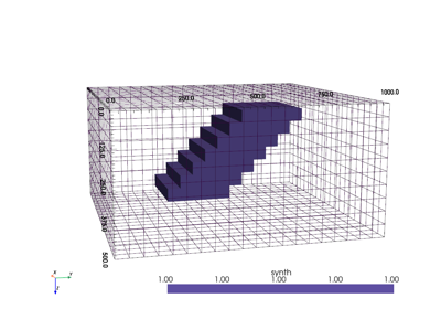
- pygimli.viewer.pv.drawMesh(ax, mesh, notebook=False, **kwargs)#
Draw a mesh into a given plotter.
- Parameters:
ax (pyvista.Plotter [optional]) – The plotter to draw everything. If none is given, one will be created.
mesh (pg.Mesh) – The mesh to show.
notebook (bool [False]) – Sets the plotter up for jupyter notebook/lab.
cMap (str ['viridis']) – The colormap string.
bc (pyvista color ['#EEEEEE']) – Background color.
style (str['surface']) – Possible options: “surface”, “wireframe”, “points”
label (str) – Data to be plotted. If None the first is taken.
- Returns:
ax – The plotter
- Return type:
pyvista.Plotter [optional]
Examples using pygimli.viewer.pv.drawMesh
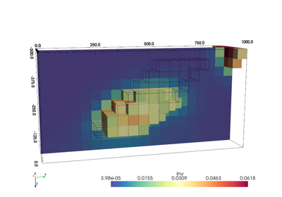
- pygimli.viewer.pv.drawModel(ax=None, mesh=None, data=None, **kwargs)#
Draw a mesh with given data.
- Parameters:
ax (pyvista.Plotter [None]) – Pyvista’s basic Plotter to add the mesh to.
mesh (pg.Mesh) – The Mesh to plot.
data (iterable) – Data that should be displayed with the mesh.
- Returns:
ax – The plotter
- Return type:
pyvista.Plotter [optional]
- pygimli.viewer.pv.drawSensors(ax, sensors, diam=0.01, color='grey', **kwargs)#
Draw the sensor positions to given mesh or the the one in given plotter.
- Parameters:
- Returns:
ax – The plotter containing the mesh and drawn electrode positions.
- Return type:
pyvista.Plotter
Examples using pygimli.viewer.pv.drawSensors
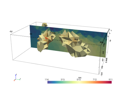
- pygimli.viewer.pv.drawSlice(ax, mesh, normal=[1, 0, 0], **kwargs)#
Draw a slice in a 3D mesh for given pygimli mesh.
- Parameters:
ax (pyvista.Plotter) – The Plotter to draw on.
mesh (pg.Mesh) – The mesh to take the slice out of.
normal (list [[1, 0, 0]]) – Coordinates to orientate the slice.
- Returns:
ax (pyvista.Plotter) – The plotter containing the mesh and drawn electrode positions.
Keyword arguments passed to pyvista.slice
—————————————–
normal ([float, float, float] | str) – normal vector constructing the slice
origin ([float, float, float]) – origin for the slice (by default mesh center)
generate_triangles (bool [False]) – generate triangle mesh
contour (bool [False]) – draw contours instead
Keyword arguments passed to pyvista.add_mesh
——————————————–
cmap|cMap (str [None]) – colormap
log_scale|logScale (bool [False]) – use logarithmic colormap scaling
clim ([float, float]) – color limits as tuple/list
cMin, cMax (float) – color limits in pg style
More information at
https (//docs.pyvista.org/api/core/_autosummary/pyvista.CompositeFilters.slice.html)
Examples using pygimli.viewer.pv.drawSlice
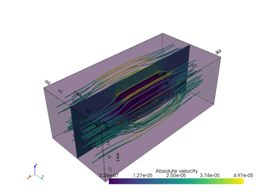
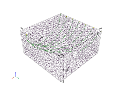
- pygimli.viewer.pv.drawStreamLines(ax, mesh, data, label=None, radius=0.01, **kwargs)#
Draw streamlines of given data.
PyVista streamline needs a vector field of gradient data per cell.
- Parameters:
ax (pyvista.Plotter [None]) – The plotter that should be used for visualization.
mesh (pyvista.UnstructuredGrid|pg.Mesh [None]) – Structure to plot the streamlines in to. If pv grid a check is performed if the data set is already contained.
data (iterable [None]) – Values used for streamlining.
label (str) – Label for the data set. Will be searched for within the data.
radius (float [0.01]) – Radius for the streamline tubes.
Note
All kwargs will be forwarded to pyvistas streamline filter: https://docs.pyvista.org/api/core/_autosummary/pyvista.DataSetFilters.streamlines.html
Examples using pygimli.viewer.pv.drawStreamLines
- pygimli.viewer.pv.pgMesh2pvMesh(mesh, data=None, label=None, boundaries=False)[source]#
pyGIMLi’s mesh format is different from pyvista’s needs, some preparation is necessary.
- Parameters:
mesh (pg.Mesh) – Structure generated by pyGIMLi to display.
data (iterable) – Parameter to distribute to cells/nodes.
- pygimli.viewer.pv.showMesh3D(mesh, data, **kwargs)[source]#
Calling the defined function to show the 3D object.
- pygimli.viewer.pv.toPVMesh(mesh, data=None, label=None, boundaries=False)#
pyGIMLi’s mesh format is different from pyvista’s needs, some preparation is necessary.
- Parameters:
mesh (pg.Mesh) – Structure generated by pyGIMLi to display.
data (iterable) – Parameter to distribute to cells/nodes.