Hydrogeophysical modeling

Coupled hydrogeophysical modeling example. This essentially represents the forward modeling step of the example presented in section 3.2 of the pyGIMLi paper.

import numpy as np

import pygimli as pg
import pygimli.meshtools as mt
import pygimli.physics.ert as ert
import pygimli.physics.petro as petro
from pygimli.physics import ERTManager

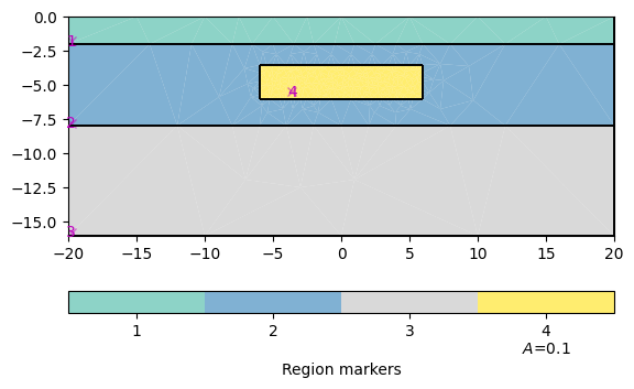
Create geometry definition for the modeling domain

world = mt.createWorld(start=[-20, 0], end=[20, -16], layers=[-2, -8],
                       worldMarker=False)

# Create a heterogeneous block
block = mt.createRectangle(start=[-6, -3.5], end=[6, -6.0], marker=4,
                           boundaryMarker=10, area=0.1)

# Merge geometrical entities
geom = world + block
pg.show(geom, boundaryMarker=True)

(<AxesSubplot:>, None)

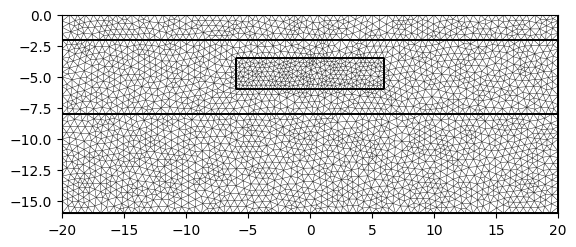
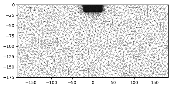
Create a mesh from the geometry definition

mesh = mt.createMesh(geom, quality=32, area=0.2, smooth=[1, 10])
pg.show(mesh)

(<AxesSubplot:>, None)

Fluid flow in a porous medium of slow non-viscous and non-frictional hydraulic movement is governed by Darcy’s Law according to:

\[\begin{split}K^{-1}\mathbf{v} + \nabla p & = 0 \\ \nabla \cdot \mathbf{v} & = 0\\ \text{leading}\,\,\text{to}\,\, \nabla\cdot(K \nabla p) & = 0 \quad \text{on} \quad\Omega\end{split}\]

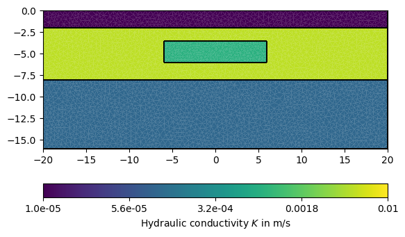
We begin by defining isotropic values of hydraulic conductivity \(K\) and mapping these to each mesh cell:

# Map regions to hydraulic conductivity in $m/s$
kMap = [[1, 1e-8], [2, 5e-3], [3, 1e-4], [4, 8e-4]]

# Map conductivity value per region to each cell in the given mesh
K = pg.solver.parseMapToCellArray(kMap, mesh)

pg.show(mesh, data=K, label='Hydraulic conductivity $K$ in m$/$s', cMin=1e-5,
        cMax=1e-2, logScale=True, grid=True)

(<AxesSubplot:>, <matplotlib.colorbar.Colorbar object at 0x7fbe6a96a6b0>)

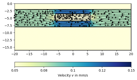
The problem further boundary conditions of the hydraulic potential. We use \(p=p_0=0.75\) m on the left and \(p=0\) on the right boundary of the modelling domain, equaling a hydraulic gradient of 1.75%.

# Dirichlet conditions for hydraulic potential
left = 0.75
right = 0.0
pBound = {"Dirichlet": {1: left, 2: left, 3: left, 5: right, 6: right, 7: right}}

We can now call the finite element solver with the generated mesh, hydraulic conductivity and the boundary condition. The sought hydraulic velocity distribution can then be calculated as the gradient field of \(\mathbf{v}=-\nabla p\) and visualized using the generic pg.show() function.

# Solve for hydraulic potential
p = pg.solver.solveFiniteElements(mesh, a=K, bc=pBound)

# Solve velocity as gradient of hydraulic potential
vel = -pg.solver.grad(mesh, p) * np.asarray([K, K, K]).T

ax, _ = pg.show(mesh, data=pg.abs(vel) * 1000, cMin=0.05, cMax=0.15,
                label='Velocity $v$ in mm$/$s', cMap='YlGnBu', hold=True)
ax, _ = pg.show(mesh, data=vel, ax=ax, color='k', linewidth=0.8, dropTol=1e-5,
                hold=True)

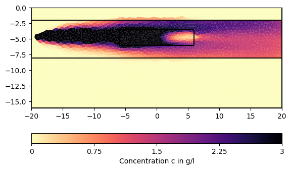
In the next step, we use this velocity field to simulate the dynamic movement of a particle (e.g., salt) concentration \(c(\mathbf{r}, t)\) in the aquifer by using the advection-diffusion equation:

\[\frac{\partial c}{\partial t} = \underbrace{\nabla\cdot(D \nabla c)}_{\text{Diffusion / Dispersion}} - \underbrace{\nabla \cdot (\mathbf{v}\nabla c)}_{\text{Advection}} + S\]

S = pg.Vector(mesh.cellCount(), 0.0)

# Fill injection source vector for a fixed injection position
sourceCell = mesh.findCell([-19.1, -4.6])
S[sourceCell.id()] = 1.0 / sourceCell.size()  # g/(l s)

We define a time vector and common velocity-depending dispersion coefficient \(D = \alpha |\mathbf{v}|\) with a dispersivity \(\alpha=1\cdot10^{-2}\) m. We solve the advection-diffsuion equation on the equation level with the finite volume solver, which results in a particle concentration :math:`c(mathbf{r},t)$ (in g/l) for each cell center and time step.

# Choose 800 time steps for 6 days in seconds
t = pg.utils.grange(0, 6 * 24 * 3600, n=800)

# Create dispersitivity, depending on the absolute velocity
dispersion = pg.abs(vel) * 1e-2

# Solve for injection time, but we need velocities on cell nodes
veln = mt.cellDataToNodeData(mesh, vel)
c1 = pg.solver.solveFiniteVolume(mesh, a=dispersion, f=S, vel=veln, times=t,
                                 scheme='PS', verbose=0)

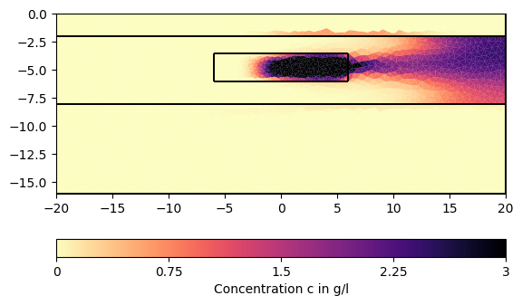
# Solve without injection starting with last result
c2 = pg.solver.solveFiniteVolume(mesh, a=dispersion, f=0, vel=veln, u0=c1[-1],
                                 times=t, scheme='PS', verbose=0)
# Stack results together
c = np.vstack((c1, c2))

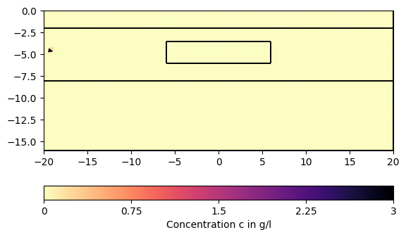
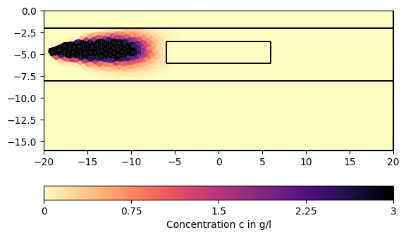
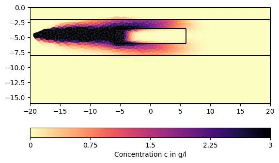
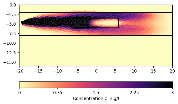
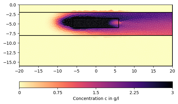
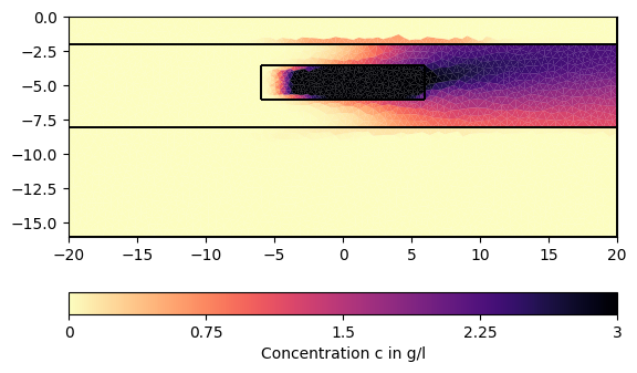
# We can now visualize the result:
for ci in c[1:][::200]:
    pg.show(mesh, data=ci * 0.001, cMin=0, cMax=3, cMap="magma_r",
            label="Concentration c in $g/l$")

• 
• 
• 
• 
• 
• 
• 
• 

/usr/lib/python3/dist-packages/scipy/sparse/linalg/_dsolve/linsolve.py:322: SparseEfficiencyWarning: splu requires CSC matrix format
  warn('splu requires CSC matrix format', SparseEfficiencyWarning)

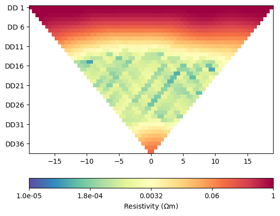
Simulate time-lapse electrical resistivity measurements.

Create a dipole-dipole measurement scheme and a suitable mesh for ERT forward simulations.

ertScheme = ert.createERTData(pg.utils.grange(-20, 20, dx=1.0), schemeName='dd')

meshERT = mt.createParaMesh(ertScheme, quality=33, paraMaxCellSize=0.2,
                            boundaryMaxCellSize=50, smooth=[1, 2])
pg.show(meshERT)

(<AxesSubplot:>, None)

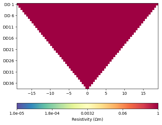
Use simulated concentrations to calculate bulk resistivity using Archie’s Law and fill matrix with apparent resistivity ratios with respect to a background model:

# Select 10 time frame to simulate ERT data
timesERT = pg.IVector(np.floor(np.linspace(0, len(c) - 1, 10)))

# Create conductivity of fluid for salt concentration $c$
sigmaFluid = c[timesERT] * 0.1 + 0.01

# Calculate bulk resistivity based on Archie's Law
resBulk = petro.resistivityArchie(rFluid=1. / sigmaFluid, porosity=0.3, m=1.3,
                                  mesh=mesh, meshI=meshERT, fill=1)

# apply background resistivity model
rho0 = np.zeros(meshERT.cellCount()) + 1000.
for c in meshERT.cells():
    if c.center()[1] < -8:
        rho0[c.id()] = 150.
    elif c.center()[1] < -2:
        rho0[c.id()] = 500.
resis = pg.Matrix(resBulk)
for i, rbI in enumerate(resBulk):
    resis[i] = 1. / ((1. / rbI) + 1. / rho0)

Initialize and call the ERT manager for electrical simulation:

ERT = ERTManager(verbose=False)
# Run  simulation for  the apparent resistivities
rhoa = ERT.simulate(meshERT, res=resis, scheme=ertScheme,
                    returnArray=True, verbose=False)

for i in range(4):
    ERT.showData(ertScheme, vals=rhoa[i]/rhoa[0], cMin=1e-5, cMax=1)

• 
• 
• 
•