Note
Go to the end to download the full example code
2D ERT modeling and inversion#
import matplotlib.pyplot as plt
import numpy as np

import pygimli as pg
import pygimli.meshtools as mt
from pygimli.physics import ert
Geometry definition#
Create geometry definition for the modelling domain. worldMarker=True
indicates the default boundary conditions for the ERT
world = mt.createWorld(start=[-50, 0], end=[50, -50], layers=[-1, -5],
                       worldMarker=True)
Create some heterogeneous circular anomaly
block = mt.createCircle(pos=[-5, -3.], radius=[4, 1], marker=4,
                        boundaryMarker=10, area=0.1)
poly = mt.createPolygon([(1,-4), (2,-1.5), (4,-2), (5,-2),
                         (8,-3), (5,-3.5), (3,-4.5)], isClosed=True,
                         addNodes=3, interpolate='spline', marker=5)
Merge geometry definition into a Piecewise Linear Complex (PLC)
geom = world + block + poly
Optional: show the geometry
pg.show(geom)
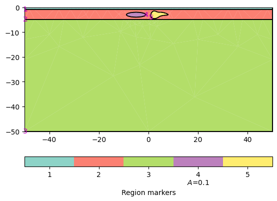
(<AxesSubplot:>, None)
Synthetic data generation#
Create a Dipole Dipole (‘dd’) measuring scheme with 21 electrodes.
scheme = ert.createData(elecs=np.linspace(start=-15, stop=15, num=21),
                           schemeName='dd')
Put all electrode (aka sensors) positions into the PLC to enforce mesh refinement. Due to experience, its convenient to add further refinement nodes in a distance of 10% of electrode spacing to achieve sufficient numerical accuracy.
for p in scheme.sensors():
    geom.createNode(p)
    geom.createNode(p - [0, 0.1])

# Create a mesh for the finite element modelling with appropriate mesh quality.
mesh = mt.createMesh(geom, quality=34)

# Create a map to set resistivity values in the appropriate regions
# [[regionNumber, resistivity], [regionNumber, resistivity], [...]
rhomap = [[1, 100.],
          [2, 75.],
          [3, 50.],
          [4, 150.],
          [5, 25]]

# Take a look at the mesh and the resistivity distribution
pg.show(mesh, data=rhomap, label=pg.unit('res'), showMesh=True)
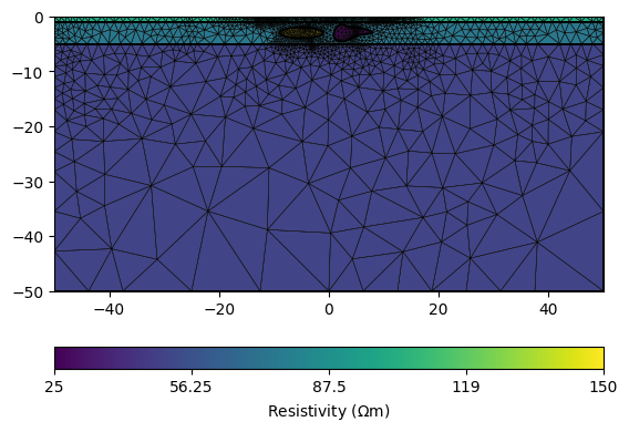
(<AxesSubplot:>, <matplotlib.colorbar.Colorbar object at 0x7fbe87d74430>)
Perform the modeling with the mesh and the measuring scheme itself and return a data container with apparent resistivity values, geometric factors and estimated data errors specified by the noise setting. The noise is also added to the data. Here 1% plus 1µV. Note, we force a specific noise seed as we want reproducable results for testing purposes.
data = ert.simulate(mesh, scheme=scheme, res=rhomap, noiseLevel=1,
                    noiseAbs=1e-6, seed=1337)

pg.info(np.linalg.norm(data['err']), np.linalg.norm(data['rhoa']))
pg.info('Simulated data', data)
pg.info('The data contains:', data.dataMap().keys())

pg.info('Simulated rhoa (min/max)', min(data['rhoa']), max(data['rhoa']))
pg.info('Selected data noise %(min/max)', min(data['err'])*100, max(data['err'])*100)
relativeError set to a value > 0.5 .. assuming this is a percentage Error level dividing them by 100
Optional: you can filter all values and tokens in the data container. Its possible that there are some negative data values due to noise and huge geometric factors. So we need to remove them.
data.remove(data['rhoa'] < 0)
pg.info('Filtered rhoa (min/max)', min(data['rhoa']), max(data['rhoa']))

# You can save the data for further use
data.save('simple.dat')

# You can take a look at the data
ert.show(data)
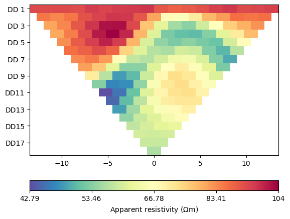
(<AxesSubplot:>, <matplotlib.colorbar.Colorbar object at 0x7fbe883e8940>)
Inversion with the ERTManager#
Initialize the ERTManager, e.g. with a data container or a filename.
mgr = ert.ERTManager('simple.dat')
Run the inversion with the preset data. The Inversion mesh will be created with default settings.
inv = mgr.invert(lam=20, verbose=True)
np.testing.assert_approx_equal(mgr.inv.chi2(), 0.7, significant=1)
fop: <pygimli.physics.ert.ertModelling.ERTModelling object at 0x7fbe872cf560>
Data transformation: <pygimli.core._pygimli_.RTransLogLU object at 0x7fbe872cf240>
Model transformation: <pygimli.core._pygimli_.RTransLog object at 0x7fbe872813a0>
min/max (data): 42.79/104
min/max (error): 1%/1.06%
min/max (start model): 67.94/67.94
--------------------------------------------------------------------------------
inv.iter 0 ... chi² =  506.26
--------------------------------------------------------------------------------
inv.iter 1 ... chi² =   14.18 (dPhi = 97.01%) lam: 20.0
--------------------------------------------------------------------------------
inv.iter 2 ... chi² =    3.05 (dPhi = 74.18%) lam: 20.0
--------------------------------------------------------------------------------
inv.iter 3 ... chi² =    0.70 (dPhi = 60.35%) lam: 20.0


################################################################################
#                  Abort criterion reached: chi² <= 1 (0.70)                   #
################################################################################
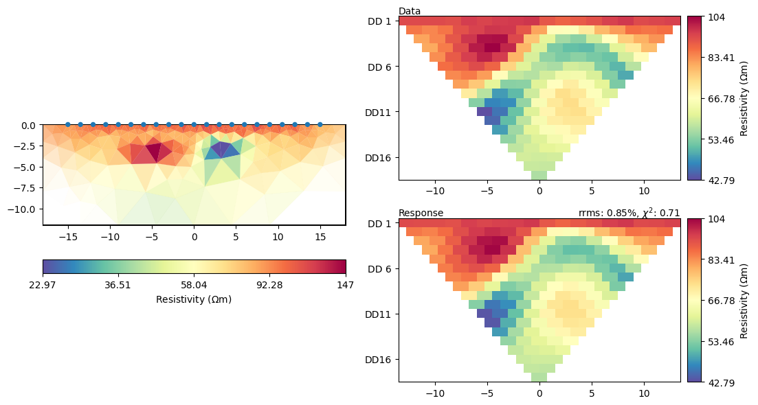
Let the ERTManger show you the model of the last successful run and how it fits the data. Shows data, model response, and model.
mgr.showResultAndFit()
meshPD = pg.Mesh(mgr.paraDomain) # Save copy of para mesh for plotting later
You can also provide your own mesh (e.g., a structured grid if you like them) Note, that x and y coordinates needs to be in ascending order to ensure that all the cells in the grid have the correct orientation, i.e., all cells need to be numbered counter-clockwise and the boundary normal directions need to point outside.
inversionDomain = pg.createGrid(x=np.linspace(start=-18, stop=18, num=33),
                                y=-pg.cat([0], pg.utils.grange(0.5, 8, n=5))[::-1],
                                marker=2)
Inversion with custom mesh#
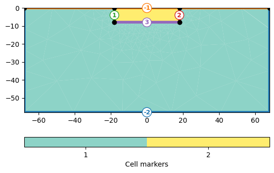
The inversion domain for ERT problems needs a boundary that represents the far regions in the subsurface of the halfspace. Give a cell marker lower than the marker for the inversion region, the lowest cell marker in the mesh will be the inversion boundary region by default.
grid = pg.meshtools.appendTriangleBoundary(inversionDomain, marker=1,
                                           xbound=50, ybound=50)
pg.show(grid, markers=True)
(<AxesSubplot:>, <matplotlib.colorbar.Colorbar object at 0x7fbe79d29cf0>)
The Inversion can be called with data and mesh as argument as well
model = mgr.invert(data, mesh=grid, lam=20, verbose=True)
fop: <pygimli.physics.ert.ertModelling.ERTModelling object at 0x7fbe872cf560>
Data transformation: <pygimli.core._pygimli_.RTransLogLU object at 0x7fbe872cf240>
Model transformation: <pygimli.core._pygimli_.RTransLog object at 0x7fbe872813a0>
min/max (data): 42.79/104
min/max (error): 1%/1.06%
min/max (start model): 67.94/67.94
--------------------------------------------------------------------------------
inv.iter 0 ... chi² =  468.39
--------------------------------------------------------------------------------
inv.iter 1 ... chi² =   77.93 (dPhi = 83.06%) lam: 20.0
--------------------------------------------------------------------------------
inv.iter 2 ... chi² =    5.37 (dPhi = 91.07%) lam: 20.0
--------------------------------------------------------------------------------
inv.iter 3 ... chi² =    2.02 (dPhi = 44.60%) lam: 20.0
--------------------------------------------------------------------------------
inv.iter 4 ... chi² =    1.51 (dPhi = 11.00%) lam: 20.0
--------------------------------------------------------------------------------
inv.iter 5 ... chi² =    1.43 (dPhi = 2.05%) lam: 20.0
--------------------------------------------------------------------------------
inv.iter 6 ... chi² =    1.42 (dPhi = 0.09%) lam: 20.0
################################################################################
#                Abort criterion reached: dPhi = 0.09 (< 2.0%)                 #
################################################################################
Visualization#
You can of course get access to mesh and model and plot them for your own. Note that the cells of the parametric domain of your mesh might be in a different order than the values in the model array if regions are used. The manager can help to permutate them into the right order.
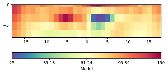
modelPD = mgr.paraModel(model) # do the mapping
pg.show(mgr.paraDomain, modelPD, label='Model', cMap='Spectral_r',
logScale=True, cMin=25, cMax=150)
pg.info('Inversion stopped with chi² = {0:.3}'.format(mgr.fw.chi2()))
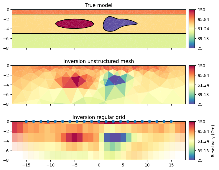
fig, (ax1, ax2, ax3) = plt.subplots(3,1, sharex=True, sharey=True, figsize=(8,7))
pg.show(mesh, rhomap, ax=ax1, hold=True, cMap="Spectral_r", logScale=True,
orientation="vertical", cMin=25, cMax=150)
pg.show(meshPD, inv, ax=ax2, hold=True, cMap="Spectral_r", logScale=True,
orientation="vertical", cMin=25, cMax=150)
mgr.showResult(ax=ax3, cMin=25, cMax=150, orientation="vertical")
labels = ["True model", "Inversion unstructured mesh", "Inversion regular grid"]
for ax, label in zip([ax1, ax2, ax3], labels):
ax.set_xlim(mgr.paraDomain.xmin(), mgr.paraDomain.xmax())
ax.set_ylim(mgr.paraDomain.ymin(), mgr.paraDomain.ymax())
ax.set_title(label)