2D crosshole ERT inversion

Inversion of 2D crosshole field data.

We import the used libraries pygimli, meshtools the ERT module and a function for displaying a data container.

import numpy as np
import pygimli as pg
import pygimli.meshtools as mt
from pygimli.physics import ert
from pygimli.viewer.mpl import showDataContainerAsMatrix

We load the data file from the example repository. It represents a crosshole data set published by Kuras et al. (2009) in the frame of the ALERT project.

data = pg.getExampleData("ert/crosshole2d.dat")
print(data)

Data: Sensors: 144 data: 1256, nonzero entries: ['a', 'b', 'err', 'm', 'n', 'r', 'valid']

There are 144 electrodes, each 16 in nine boreholes, and 1256 data that are resistances only. Therefore we first compute the geometric factors and then the apparent resistivities, of which we plot the last few values.

data["k"] = ert.geometricFactors(data, dim=3)
data["rhoa"] = data["r"] * data["k"]
print(np.sort(data["rhoa"])[-5:])

[181.85035034 192.9622767  210.49617346 258.10205765 537.70069201]

We see that there is a single value above 500 Ohmm and a few other high ones. Therefore we delete the highest value. We plot the data in form of a crossplot between the A and M electrodes (with forward and backward sign).

data.remove(data["rhoa"] > 200)
m = np.sign(data["m"] - data["n"]) * data["m"]
showDataContainerAsMatrix(data, m, data["a"], "rhoa", cMap="Spectral_r")

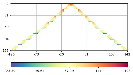
(<AxesSubplot:>, <matplotlib.colorbar.Colorbar object at 0x7fbe89533df0>)

We determine the x and z positions and create a regular grid with a spacing of 5xm that contains the electrodes as nodes. This is not necessary but improves quality of the forward response. Around the boreholes there is 0.5m space and all mesh cells have the marker 2.

ex = np.unique(pg.x(data))
ez = np.unique(pg.z(data))
dx = 0.1
nb = 4
xmin, xmax = min(ex) - nb*dx, max(ex) + nb*dx
zmin, zmax = min(ez) - nb*dx, 0
x = np.arange(xmin, xmax+.001, dx)
z = np.arange(zmin, zmax+.001, dx)
grid = mt.createGrid(x, z, marker=2)
ax, cb = pg.show(grid, showMesh=True, markers=True)
ax.plot(pg.x(data), pg.z(data), "mx")
print(grid)

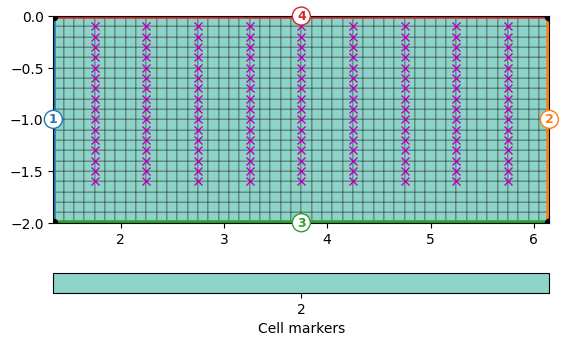
Mesh: Nodes: 1029 Cells: 960 Boundaries: 1988

In order to ensure correct boundary conditions, we append a triangular mesh outside that is automatically treated as background because they have a region marker of 1 and so-called world boundary conditions, i.e. Neumann BC at the Earth’s surface and mixed boundary conditions at the other boundaries. Additionally, we give all the boundaries at a specific depth a marker > 0 so that this is treated as known interface where smoothness does not apply.

mesh = mt.appendTriangleBoundary(grid, marker=1, boundary=4, worldMarkers=True)
for b in mesh.boundaries():
    if np.isclose(b.center().y(), -1.7):
        b.setMarker(1)

# pg.show(mesh, markers=True)

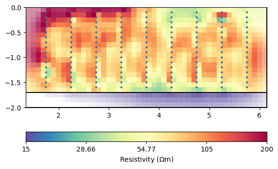
We estimate an error using default values, i.e. 3% relative error and an absolute error of 100uV at an assumed current of 100mA which is almost zero. Inversion is run with half as much weight into the vertical direction.

data.estimateError()
mgr = ert.Manager(data)
mgr.invert(mesh=mesh, verbose=True)
mgr.showResult(cMin=15, cMax=200)

fop: <pygimli.physics.ert.ertModelling.ERTModelling object at 0x7fbe780623e0>
Data transformation: <pygimli.core._pygimli_.RTransLogLU object at 0x7fbe780b4860>
Model transformation: <pygimli.core._pygimli_.RTransLog object at 0x7fbe873371a0>
min/max (data): 23.39/193
min/max (error): 3%/3%
min/max (start model): 68.62/68.62
--------------------------------------------------------------------------------
inv.iter 0 ... chi² =  107.27
--------------------------------------------------------------------------------
inv.iter 1 ... chi² =   21.39 (dPhi = 78.94%) lam: 20.0
--------------------------------------------------------------------------------
inv.iter 2 ... chi² =    4.74 (dPhi = 74.64%) lam: 20.0
--------------------------------------------------------------------------------
inv.iter 3 ... chi² =    4.39 (dPhi = 6.02%) lam: 20.0
--------------------------------------------------------------------------------
inv.iter 4 ... chi² =    3.31 (dPhi = 13.06%) lam: 20.0
--------------------------------------------------------------------------------
inv.iter 5 ... chi² =    2.70 (dPhi = 13.22%) lam: 20.0
--------------------------------------------------------------------------------
inv.iter 6 ... chi² =    2.64 (dPhi = 0.74%) lam: 20.0
################################################################################
#                Abort criterion reached: dPhi = 0.74 (< 2.0%)                 #
################################################################################

(<AxesSubplot:>, <matplotlib.colorbar.Colorbar object at 0x7fbe7afa5390>)

References

Kuras, O., Pritchard, J., Meldrum, P. I., Chambers, J. E., Wilkinson, P. B., Ogilvy, R. D.,and Wealthall, G. P. (2009). Monitoring hydraulic processes with Automated time-Lapse Electrical Resistivity Tomography (ALERT). Compte Rendus Geosciences - Special issue on Hydrogeophysics, 341(10-11):868–885.