3D crosshole ERT inversion

In this example, we demonstrate the inversion of 3D crosshole field data. Instead of a regular grid or an irregular tetrahedral mesh, we use triangular prism mesh (triangles in x-y plane and regular along z). This is beneficial in cases of a predominant layering that can be accounted for by using the zWeight inversion parameter because the boundaries are perfectly vertical.

We import the used libraries pygimli, meshtools the ERT module and a function for displaying a data container.

import numpy as np
import pygimli as pg
import pygimli.meshtools as mt
from pygimli.physics import ert
from pygimli.viewer.mpl import showDataContainerAsMatrix

We load the data file from the example repository. It represents a crosshole data set published by Doetsch et al. (2010) in the frame of the RECORD project where boreholes were installed to monitor the exchange between river and groundwater (Coscia et al., 2008).

data = pg.getExampleData("ert/crosshole3d.dat")
print(data)

Data: Sensors: 36 data: 753, nonzero entries: ['a', 'b', 'm', 'n', 'r', 'valid']

There are 36 electrodes, each 9 in four boreholes, and 1256 data that are resistances only. Therefore we first compute the geometric factors and then the apparent resistivities, of which we plot the last few values.

data["k"] = ert.geometricFactors(data, dim=3)
data["rhoa"] = data["r"] * data["k"]

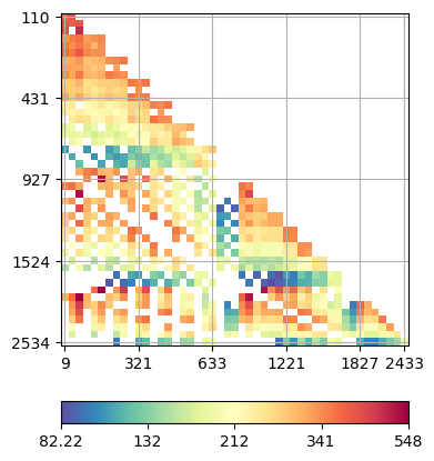
We plot the data in form of a crossplot between the A-B and M-N electrode combinations. Values are in the range between 100 and 500 Ohmmeters.

ab = data["a"] * 100 + data["b"]
mn = data["m"] * 100 + data["n"]
ax, cb = showDataContainerAsMatrix(data, ab, mn, "rhoa", cMap="Spectral_r")

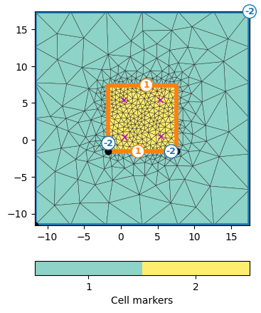
We first extract the borehole locations, i.e. the x and y positions of the electrodes. From these we create a rectangle with 40% boundary and marker 2 and add the borehole positions to it.

elPosXY = np.unique(np.column_stack([pg.x(data), pg.y(data)]), axis=0)
rect = mt.createRectangle(pnts=elPosXY, minBBOffset=1.4, marker=2)
for elpos in elPosXY:
    rect.createNode(*elpos, 0)

# ax, cb = pg.show(rect)
# _ = ax.plot(*elPosXY.T, "mx")

From this PLC, we create a mesh using a maximum cell size. We add an outer (modelling) boundary.

bnd = 5
rectMesh = mt.createMesh(rect, quality=34.3, area=.4)
mesh2d = mt.appendTriangleBoundary(
    rectMesh, boundary=bnd, isSubSurface=False, marker=1)
ax, cb = pg.show(mesh2d, markers=True, showMesh=True)
_ = ax.plot(*elPosXY.T, "mx")

We create a vertical discretization vector with dense spacing in the range of the electrodes and a coarser discretization above and below.

dTop, dBot = 4.1, 10.1
dzIn, dzOut = 0.4, 0.8
zTop = np.arange(0, dTop, dzOut)  # the upper layer
zMid = np.arange(zTop[-1], dBot, dzIn)  # the middle
zBot = np.arange(zMid[-1], dBot+bnd+.1, dzOut)  # the lower layer
zVec = -np.concatenate([zTop, zMid[1:], zBot[1:]])  # all vectors together
print(zVec)

[ -0.   -0.8  -1.6  -2.4  -3.2  -4.   -4.4  -4.8  -5.2  -5.6  -6.   -6.4
  -6.8  -7.2  -7.6  -8.   -8.4  -8.8  -9.2  -9.6 -10.  -10.8 -11.6 -12.4
 -13.2 -14.  -14.8]

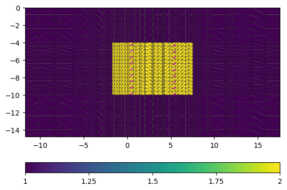
From the 2d mesh and the z vector we create a 3D triangular prism mesh that obtains the marker of the 2D mesh. Additionally, we set all cells above or below to marker 1 which is by default the background region. In total we have 56k cells, of which most are background and less than 20k cells are inverted.

mesh = mt.createMesh3D(mesh2d, zVec, pg.core.MARKER_BOUND_HOMOGEN_NEUMANN,
                       pg.core.MARKER_BOUND_MIXED)
print(mesh)
for c in mesh.cells():
    cd = -c.center().z()  # center depth
    if cd < dTop or cd > dBot:
        c.setMarker(1)

mesh["region"] = pg.Vector(mesh.cellMarkers())
sli = mt.extract2dSlice(mesh)
ax, cb = pg.show(sli, "region", showMesh=True)
_ = ax.plot(pg.x(data), pg.z(data), "mo", markersize=1)

Mesh: Nodes: 11664 Cells: 21736 Boundaries: 3830

We estimate an error using default values, i.e. 3% relative error and an absolute error of 100uV at an assumed current of 100mA which is almost zero. Inversion is run with less weight into the vertical direction.

data["err"] = ert.estimateError(data)
mgr = ert.Manager(data)
mgr.invert(mesh=mesh, zWeight=0.3, verbose=True)

fop: <pygimli.physics.ert.ertModelling.ERTModelling object at 0x7fbe78393ec0>
Data transformation: <pygimli.core._pygimli_.RTransLogLU object at 0x7fbe79cef6f0>
Model transformation (cumulative):
         0 <pygimli.core._pygimli_.RTransLogLU object at 0x7fbe7b062200>
min/max (data): 82.22/548
min/max (error): 3%/3%
min/max (start model): 243/243
--------------------------------------------------------------------------------
inv.iter 0 ... chi² =  160.94
--------------------------------------------------------------------------------
inv.iter 1 ... chi² =   15.07 (dPhi = 89.62%) lam: 20.0
--------------------------------------------------------------------------------
inv.iter 2 ... chi² =    3.53 (dPhi = 61.66%) lam: 20.0
--------------------------------------------------------------------------------
inv.iter 3 ... chi² =    2.20 (dPhi = 22.88%) lam: 20.0
--------------------------------------------------------------------------------
inv.iter 4 ... chi² =    1.57 (dPhi = 8.35%) lam: 20.0
--------------------------------------------------------------------------------
inv.iter 5 ... chi² =    1.55 (dPhi = 0.59%) lam: 20.0
################################################################################
#                Abort criterion reached: dPhi = 0.59 (< 2.0%)                 #
################################################################################

6015 [326.69003711091324,...,140.94783118836844]

Eventually, we are able to fit the data to a chi-square value close to 1, or about 3% RRMS. We visualize the result using the pyVista package with a clip. The electrodes are marked by magenta points. We mainly see a layering with highest resistivity on top and lowest at the bottom.

pd = mgr.paraDomain
pd["res"] = mgr.model
pl, _ = pg.show(pd, label="res", style="surface", cMap="Spectral_r", hold=1,
                filter={"clip": dict(normal=[1, 1, 0], origin=[2, 2, -6])})
pl.add_points(data.sensors().array(), color="magenta")
pl.camera_position = "yz"
pl.camera.azimuth = 20
pl.camera.elevation = 20
pl.camera.zoom(1.2)
_ = pl.show()

/usr/local/lib/python3.10/dist-packages/pyvista/plotting/themes.py:2942: PyVistaDeprecationWarning: `DefaultTheme` has been deprecated and renamed `Theme`. Further, `DocumentTheme` is now the PyVista default theme.
  warnings.warn(

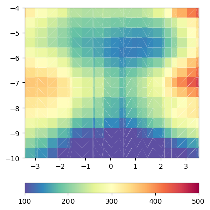
We also have a closer look at a slice through the middle.

para = mgr.paraDomain
para["res"] = mgr.paraModel()
slice = mt.extract2dSlice(para, origin=[4, 4, 0], normal=[1, 1, 0])
pg.show(slice, "res", cMap="Spectral_r", cMin=100, cMax=500)

(<AxesSubplot:>, <matplotlib.colorbar.Colorbar object at 0x7fbe864f44f0>)

References

Coscia, I., S. Greenhalgh, N. Linde, A. Green, T. Günter, J. Doetsch, and T. Vogt, 2010, A multi-borehole 3-D ERT monitoring system for aquifer characterization using river flood events as a natural tracer: Ext. Abstr. 16th Annual EAGE meeting of Environmental and Engineering Geophysics.

Doetsch, J., Linde, N., Coscia, I., Greenhalgh, S., & Green, A. (2010): Zonation for 3D aquifer characterization based on joint inversions of multimethod crosshole geophysical data. GEOPHYSICS (2010),75(6): G53.