Note
Go to the end to download the full example code
Geoelectrics in 2.5D#
This example shows geoelectrical (DC resistivity) forward modelling in 2.5 D, i.e. a 2D conductivity distribution and 3D point sources, to illustrate the modeling level. For ready-made ERT forward simulations in practice, please refer to the example on ERT modeling and inversion using the ERTManager.
Let us start with the gouverning partial differential equation of Poisson type
The source term (point electrode) is three-dimensional, but the distribution of the electrical conductivity \(\sigma(x,y)\) should be 2D so we apply a Fourier cosine transform from \(u(x,y,z) \mapsto u(x,k,z)\) with the wave number \(k\). (\(D^{(a)}(u(x,y,z)) \mapsto i^{|a|}k^a u(x,z)\))
import matplotlib
import numpy as np
import pygimli as pg

from pygimli.viewer.mpl import drawStreams
We know the exact solution by analytical formulas:
with K0 being the Bessel function of first kind, and the normal and mirror sources r+ and r-. We define a function for it
def uAnalytical(p, sourcePos, k, sigma=1):
    """Calculates the analytical solution for the 2.5D geoelectrical problem.

    Solves the 2.5D geoelectrical problem for one wave number k.
    It calculates the normalized (for injection current 1 A and sigma=1 S/m)
    potential at position p for a current injection at position sourcePos.
    Injection at the subsurface is recognized via mirror sources along the
    surface at depth=0.

    Parameters
    ----------
    p : pg.Pos
        Position for the sought potential
    sourcePos : pg.Pos
        Current injection position.
    k : float
        Wave number

    Returns
    -------
    u : float
        Solution u(p)
    """
    r1A = (p - sourcePos).abs()
    # Mirror on surface at depth=0
    r2A = (p - pg.Pos([1.0, -1.0])*sourcePos).abs()

    if r1A > 1e-12 and r2A > 1e-12:
        return  1 / (2.0 * np.pi) * 1/sigma * \
            (pg.math.besselK0(r1A * k) + pg.math.besselK0(r2A * k))
    else:
        return 0.
We assume the so-called mixed boundary conditions (Dey & Morrison, 1979).
def mixedBC(boundary, userData):
    """Mixed boundary conditions.

    Define the derivative of the analytical solution regarding the outer normal
    direction :math:`\vec{n}`. So we can define the values for mixed boundary
    condition :math:`\frac{\partial u}{\partial \vec{n}} = -au`
    for the boundaries on the subsurface.

    """
    ### ignore surface boundaries for wildcard boundary condition
    if boundary.norm()[1] == 1.0:
        return 0

    sourcePos = userData['sourcePos']
    k = userData['k']
    sigma = userData['s']
    r1 = boundary.center() - sourcePos

    # Mirror on surface at depth=0
    r2 = boundary.center() - pg.Pos(1.0, -1.0) * sourcePos
    r1A = r1.abs()
    r2A = r2.abs()

    n = boundary.norm()
    if r1A > 1e-12 and r2A > 1e-12:
        alpha = sigma * k * ((r1.dot(n)) / r1A * pg.math.besselK1(r1A * k) +
                            (r2.dot(n)) / r2A * pg.math.besselK1(r2A * k)) / \
            (pg.math.besselK0(r1A * k) + pg.math.besselK0(r2A * k))

        return alpha

        # Note, the above is the same like:
        beta = 1.0
        return [alpha, beta, 0.0]

    else:
        return 0.0
We assemble the right-hand side (rhs) for the singular current term by hand since this cannot be done efficiently by pg.solve yet. We basically search for the cell containing the source and project the point using its shape functions N.
def rhsPointSource(mesh, source):
    """Define function for the current source term.

    :math:`\delta(x-pos), \int f(x) \delta(x-pos)=f(pos)=N(pos)`
    Right hand side entries will be shape functions(pos)
    """
    rhs = pg.Vector(mesh.nodeCount())

    cell = mesh.findCell(source)
    rhs.setVal(cell.N(cell.shape().rst(source)), cell.ids())
    return rhs
Now we create a suitable mesh and solve the equation with pg.solve. Note that we use a mesh with quadratic shape functions by calling createP2.
mesh = pg.createGrid(x=np.linspace(-10.0, 10.0, 41),
y=np.linspace(-15.0, 0.0, 31))
mesh = mesh.createP2()
sourcePosA = [-5.25, -3.75]
sourcePosB = [+5.25, -3.75]
k = 1e-2
sigma = 1.0
bc={'Robin': {'1,2,3': mixedBC}}
u = pg.solve(mesh, a=sigma, b=-sigma * k*k,
rhs=rhsPointSource(mesh, sourcePosA),
bc=bc, userData={'sourcePos': sourcePosA, 'k': k, 's':sigma},
verbose=True)
u -= pg.solve(mesh, a=sigma, b=-sigma * k*k,
rhs=rhsPointSource(mesh, sourcePosB),
bc=bc, userData={'sourcePos': sourcePosB, 'k': k, 's':sigma},
verbose=True)
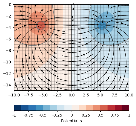
# The solution is shown by calling
ax = pg.show(mesh, data=u, cMap="RdBu_r", cMin=-1, cMax=1,
orientation='horizontal', label='Potential $u$',
nCols=16, nLevs=9, showMesh=True)[0]
# Additionally to the image of the potential we want to see the current flow.
# The current flows along the gradient of our solution and can be plotted as
# stream lines. By default, the drawStreams method draws one segment of a
# stream line per cell of the mesh. This can be a little confusing for dense
# meshes so we can give a second (coarse) mesh as a new cell base to draw the
# streams. If `drawStreams` gets scalar data, the gradients will be calculated.
gridCoarse = pg.createGrid(x=np.linspace(-10.0, 10.0, 20),
y=np.linspace(-15.0, .0, 20))
drawStreams(ax, mesh, u, coarseMesh=gridCoarse, color='Black')
Mesh:  Mesh: Nodes: 3741 Cells: 1200 Boundaries: 2470
Assembling time:  0.026669962
Solving time:  0.041520901
Mesh:  Mesh: Nodes: 3741 Cells: 1200 Boundaries: 2470
Assembling time:  0.025246523
Solving time:  0.025073414
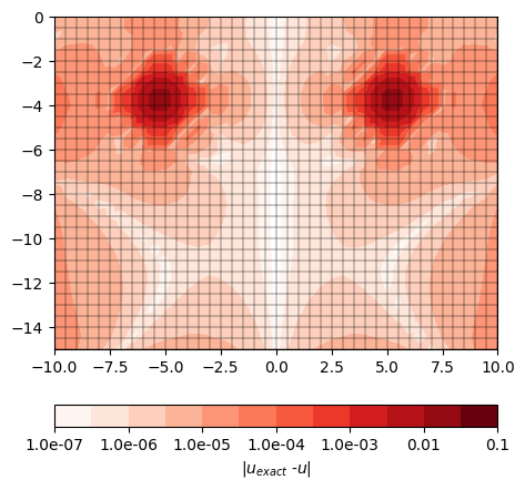
We know the exact solution so we can compare it to the numerical results. Unfortunately, the point source singularity does not allow a good integration measure for the accuracy of the resulting field so we just look for the differences.
uAna = pg.Vector(list(map(lambda p__: uAnalytical(p__, sourcePosA, k, sigma),
                      mesh.positions())))
uAna -= pg.Vector(list(map(lambda p__: uAnalytical(p__, sourcePosB, k, sigma),
                       mesh.positions())))

ax = pg.show(mesh, data=pg.abs(uAna-u), cMap="Reds",
          orientation='horizontal', label='|$u_{exact}$ -$u$|',
          logScale=True, cMin=1e-7, cMax=1e-1,
          contourLines=False,
          nCols=12, nLevs=7,
          showMesh=True)[0]

#print('l2:', pg.pf(pg.solver.normL2(uAna-u)))
print('L2:', pg.pf(pg.solver.normL2(uAna-u, mesh)))
print('H1:', pg.pf(pg.solver.normH1(uAna-u, mesh)))
np.testing.assert_approx_equal(pg.solver.normL2(uAna-u, mesh),
                               0.02415, significant=3)
L2: 0.02
H1: 0.19