2D FEM modelling on two-layer example

Compare 2D FEM modelling with 1D VES sounding with and without complex resistivity values.

import numpy as np

import pygimli as pg
import pygimli.meshtools as mt
from pygimli.physics import ert
from pygimli.physics.ves import VESModelling, VESCModelling

First we create a data configuration of a 1D Schlumberger sounding with 20 electrodes and and increasing MN/2 electrode spacing from 1m to 24m.

scheme = ert.createData(pg.utils.grange(start=1, end=24, dx=1, n=10, log=True),
                        sounding=True)

First we create a geometry that covers the sought geometry. We start with a 2 dimensional simulation world of a bounding box [-200, -100] [200, 0], the layer at -5m and some suitable requested cell sizes.

plc = mt.createWorld(start=[-200, -100], end=[200, 0],
                     layers=[-10], area=[5.0, 500])

To achieve a necessary numerical accuracy, we need some local mesh refinement in the vicinity of the electrodes. However, since we don’t need the electrode (aka sensor) positions to be present as nodes in the geometry, we only add forced mesh nodes near the electrode positions, right below the earths surface.

for s in scheme.sensors():
    plc.createNode(s + [0.0, -0.2])

# Now we can create our forward modeling mesh.
mesh = mt.createMesh(plc, quality=33)

pg.show(mesh, data=mesh.cellMarkers(), label='Marker', showMesh=True)

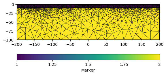
(<AxesSubplot:>, <matplotlib.colorbar.Colorbar object at 0x7fbe78256a40>)

It is usually a good idea to calculate with a p2-refined mesh. However, you should be careful for larger meshes since the numerical efford will be highly increased.

mesh = mesh.createP2()

Perform the modeling using the static convenience call for ERT. Res is the resistivity mapping regarding the regions of the given geometry. Region with marker 1 is the upper layer, maker 2 is the background

data = ert.simulate(mesh, res=[[1, 100.0], [2, 1.0]],
                   scheme=scheme, verbose=False)

1D VES

x = pg.x(scheme)
ab2 = (x[scheme('b')] - x[scheme('a')])/2
mn2 = (x[scheme('n')] - x[scheme('m')])/2
ves = VESModelling(ab2=ab2, mn2=mn2)

Plot results

fig, ax = pg.plt.subplots(1, 1)
ax.plot(ab2, data('rhoa'), '-o', label='2D (FEM)')
ax.plot(ab2, ves.response([10.0, 100.0, 1.0]), '-x', label='1D (VES)')
ax.set_xlabel('AB/2 (m)')
ax.set_ylabel('Apparent resistivity ($\Omega$m)')
ax.grid(1)
ax.legend()

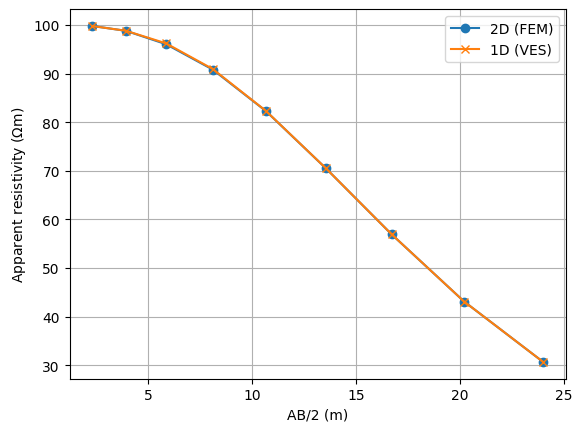
<matplotlib.legend.Legend object at 0x7fbe899caad0>

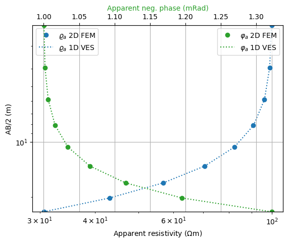
We can easily repeat the above example using a complex resistivity model. defining amplitude and phase in negative mrad.

amps = np.array([100.0, 1.0])
phases = np.array([1.0, 10.0])
res = amps - 1j * amps * np.sin(phases/1000.)
data = ert.simulate(mesh, res=[[1, res[0]], [2, res[1]]],
                   scheme=scheme, verbose=False)

ves = VESCModelling(ab2=ab2, mn2=mn2)
rc = ves.response([10.0, 100.0, 1.0, phases[0]/1000, phases[1]/1000])

We can apply the default drawing routines for 1D VES data as well.

fig, ax = pg.plt.subplots(1, 1)
ves.drawData(ax, pg.cat(data('rhoa'), -data('phia')),
            labels=[r'$\varrho_a$ 2D FEM', r'$\varphi_a$ 2D FEM'],
            marker='o', linestyle='none')
ves.drawData(ax, rc,
             labels=[r'$\varrho_a$ 1D VES', r'$\varphi_a$ 1D VES'],
             marker=None)

np.testing.assert_approx_equal(data('rhoa')[0], 30.66351249, significant=5)
np.testing.assert_approx_equal(-data('phia')[0], 0.00132173865, significant=5)