Note
Go to the end to download the full example code
CAD to mesh tutorial#
In this example you will learn how to create a geometry in FreeCAD and then export and mesh it using Gmsh.
Gmsh comes with a build-in CAD engine for defining a geometry, as shown in the flexible mesh generation example, but using a parametric CAD program such as FreeCAD is much more intuitive and flexible.
For this tutorial you will need Gmsh and its Python API (application programming interface). These can be installed by the command below inside your (new) conda environment.
conda install -c conda-forge gmsh python-gmsh
In case you also want to try out FreeCAD, installing it from their website will give you the most up to date version.
This example is based on an ERT modelling and inversion experiment on a small dike. However, this FreeCAD → Gmsh workflow can easily be translated to other geophysical methods. The geometry and acquisition design come from the IDEA League master thesis of Joost Gevaert. The target in this example is to find the geometry of a sand channel underneath the dike.
FreeCAD: create the geometry#
Two geometries have to be created. One for modelling and one for inversion. When the same meshes are used for modelling and inversion, the geometry of the sand channel is alreadyincluded in the structure of the mesh. Therefore, the mesh itself would act as prior information to the inversion. The modelling geometry consists of three regions: the outer region; the inner region (same as inversion region in this example) and the sand channel. The inversion geometry consists of two regions: the outer region and the inversion region.
The geometries are defined in three steps:
Each region of the geometry designed separately in the Part workbench, or in the Part Design workbench for more complicated geometries. To get familiar with the part design workbench, this FreeCAD-tutorial with some videos is great.
Merge all regions into one single ”compsolid”, i.e.composite solid. Meaning one object that consists of multiple solids that share the interfaces between the solids.
Export the geometry in
.brep*
(1) The outer and inversion regions of this dike example were created in the Part Design workbench, by making a sketch and then extruding it with the Pad option. See the Inversion-Region in the object tree in the figure below. You can also have a look at how these geometries were created by downloading the .FCStd FreeCAD files and playing around with them. The sand channel is a simple cube, created in the Part workbench. Dimensions: L = 8.0 m ; W = 15.0 m ; H = 2.0 m. Position: x = 7.5 m ; y = -1.5 m ; z = -2.3 m.
(2) The trick then lies in merging these shapes into a single compsolid. This is done in the following steps:
Open a new project and merge all objects, i.e. regions (File → Merge project…) into this project
In the Part workbench, select all objects and create Boolean Fragments (Part → Split → Boolean Fragments)
Select the newly created BooleanFragments in the object tree and change its Mode property to CompSolid, see the figure below.
Keep BooleanFragments selected and then apply a Compound Filter to it (Part → Compound → Compound Filter)
Quality check the obtained geometry. Select the newly created CompoundFilter from the object tree and click Check Geometry (Part → Check Geometry). SOLID: in the Shape Content, should match the number of objects merged when creating the Boolean Fragments, 3 in this example. COMPSOLID: should be 1. Always, also for other geometries. COMPOUND: should be 0. Always. COMPSOLID: 1 and COMPOUND: 0 indicates that the objects were indeed merged correctly to one single compsolid, see the figure below.
(3) Select the CompounSolid from the object tree and export (File → Export…) as .brep.
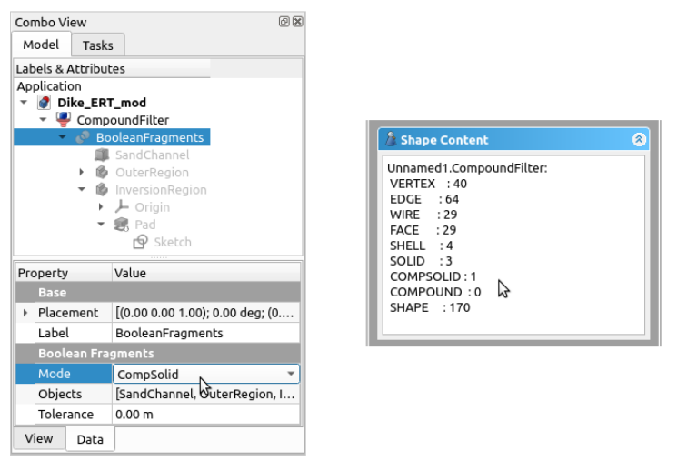
FreeCAD important dialogs for making a correct compsolid.#
It must be
.brep. This is the native format of the OpenCascade
CAD engine on which both FreeCAD and Gmsh run. .step (also
.stp) is the standardized CAD exchange format, for some reason
this format does not export the shape as a compound solid. Gmsh can
also read .stl and .iges files. .stl files only contain
surface information and cannot easily be reedited. .iges is an
old format for which development stopped after 1996 and geometries
are not always imported correctly.
Gmsh: mesh the geometry#
Meshing with Gmsh is incredibly versatile, but has a very steep learning curve. Here we use the Python Application Programming Interface (API). To get familiar with the Python API, the Gmsh tutorials (overview) were converted to Python scripts and additional demos are also provided. I will mention or provide links to relevant tutorials and demos, have a look at these for extra context.
Let’s start by importing our geometry into Gmsh:
import numpy as np
import pygimli as pg
gmsh = pg.optImport("gmsh", "do this tutorial. Install by running: pip install gmsh")

# Download all nessesary files
geom_filename = pg.getExampleFile("cad/dike_mod.brep")
elec_pos_filename = pg.getExampleFile("cad/elec_pos.csv")

if gmsh:
    # Starting it up (tutorial t1.py)
    gmsh.initialize()
    gmsh.option.setNumber("General.Terminal", 1)
    gmsh.model.add("dike_mod")
    # Load a BREP file (t20.py & demo step_assembly.py)
    # .brep files don't contain info about units, so scaling has to be applied
    gmsh.option.setNumber("Geometry.OCCScaling", 0.001)
    volumes = gmsh.model.occ.importShapes(geom_filename)
Before diving into local mesh refinement, putting the electrodes in the mesh and assigning region, boundary and electrode markers, the .brep geometry file should be checked. Especially check whether the meshes of two adjacent regions share nodes on their interfaces. The mesh can be viewed by running the following lines of code:
# Run this code after every change in the mesh to see what changed.
gmsh.model.occ.synchronize()
gmsh.model.mesh.generate(3)
gmsh.fltk.run()
Tips for viewing the mesh:
Double left clicking opens a menu in where you can set geometry and mesh visibility.
Tools → Visibility opens a window in which you can select parts of the mesh and geometry. Here you can find the tags of the elementary entities of the geometry. It is also handy later to QC whether physical groups were set correctly.
Clip the mesh and geometry with Tools → Clipping.
The number of elements ect. can be found in the Tools → Statistics window.
Make sure to quickly write down the Gmsh volume tags of the outer region, dike and channel and the surface tags of the free surface and the underground boundary of the box. You will need this in the next step.
If importing and meshing the .brep geometry went correctly, great! Next we include the electrodes (from Excel file) into the geometry and define the Characteristic Length (CL) for each region and the electrodes. The CL is defined at each Point and dictates the mesh size at that point. The mesh size between points is interpolated linearly, by default.
cl_elec = 0.1
cl_dike = 0.6
cl_outer = 30
# Gmsh geometry tags of relevant parts. Find the tags in the Gmsh interface.
tags = {"outer region": 2,
    "dike": 3,
    "channel": 1,
    "surface": [7, 11, 12, 13, 21, 23, 24,
                25, 27, 29, 30, 31],
    "boundary": [8, 14, 15, 16, 20],      # "Underground Box Boundary"
    "electrodes": []}

if gmsh:
    # Syncronize CAD representation with the Gmsh model (t1.py)
    # Otherwise gmsh.model.get* methods don't work.
    gmsh.model.occ.synchronize()
    # Set mesh sizes for the dike and outer region.
    # The order, in which mesh sizes are set, matters. Big -> Small
    gmsh.model.mesh.setSize(              # Especially t16.py, also t2; 15; 18; 21
        gmsh.model.getBoundary(           # get dimTags of boundary elements of
            [(3, tags["outer region"])],  # dimTag: (dim, tag)
            recursive=True),              # recursive -> dimTags of points
        cl_outer)
    gmsh.model.mesh.setSize(
        gmsh.model.getBoundary([(3, tags["dike"])],recursive=True),
        cl_dike)
Now reload the script, mesh the geometry again and have a look how the mesh changed. The next step is adding the electrodes to the mesh. The grid on the dike has 152 electrodes. These points are added in Gmsh as points 201-352, to prevent clashing with points already defined in the geometry.
if gmsh:
    # positions: np.array([elec#, x, y, z, y "over ground"])
    pos = np.genfromtxt(elec_pos_filename, delimiter=",", skip_header=1)
    # Electrodes are put at 2 cm depth, such that they can be embeded in the volume of the dike.
    # Embeding the electrodes into the surface elements complicates meshing.
    elec_depth = 0.02               # elec depth [m]
    pos[:, 3] = pos[:, 3] - elec_depth
    # Add the electrodes to the Gmsh model and put the tags into the Dict
    for xyz in pos:
        tag = int(200 + xyz[0])
        gmsh.model.occ.addPoint(xyz[1], xyz[2], xyz[3], cl_elec, tag)
        tags["electrodes"].append(tag)
    # Embed electrodes in dike volume. (t15.py)
    gmsh.model.occ.synchronize()
    gmsh.model.mesh.embed(0, tags["electrodes"], 3, tags["dike"])
Reload the Gmsh script and mesh it again to see the result. Further mesh refinement is then possible with so-called background fields. Taking a quick look at Gmsh tutorial t10.geo is highly recommended. It shows a wide range of possible background fields. In this example a Distance field is defined from the electrodes and then a Threshold field is applied as the background field:
# LcMax -                         /------------------
#                               /
#                             /
#                           /
# LcMin -o----------------/
#        |                |       |
#      Point           DistMin DistMax
# Field 1: Distance to electrodes

if gmsh:
    gmsh.model.mesh.field.add("Distance", 1)
    gmsh.model.mesh.field.setNumbers(1, "NodesList", tags["electrodes"])
    # Field 2: Threshold that dictates the mesh size of the background field
    gmsh.model.mesh.field.add("Threshold", 2)
    gmsh.model.mesh.field.setNumber(2, "IField", 1)
    gmsh.model.mesh.field.setNumber(2, "LcMin", cl_elec)
    gmsh.model.mesh.field.setNumber(2, "LcMax", cl_dike)
    gmsh.model.mesh.field.setNumber(2, "DistMin", 0.2)
    gmsh.model.mesh.field.setNumber(2, "DistMax", 1.5)
    gmsh.model.mesh.field.setNumber(2, "StopAtDistMax", 1)
    gmsh.model.mesh.field.setAsBackgroundMesh(2)
Again reload the Gmsh script and mesh it, to see the result. As the
last step in creating the mesh, the physical groups have to be
defined, such PyGIMLi recognize regions, boundaries and the
electrodes, see help(pg.meshtools.readGmsh). Make sure to follow
the same Physical Group tag number conventions for marking the
regions, surfaces and points as used in PyGIMLi.
if gmsh:
    # Physical Volumes, "Regions" in pyGIMLi
    pgrp = gmsh.model.addPhysicalGroup(3, [tags["outer region"]], 1)  #(dim, tag, pgrp tag)
    gmsh.model.setPhysicalName(3, pgrp, "Outer Region")     # Physical group name in Gmsh
    pgrp = gmsh.model.addPhysicalGroup(3, [tags["dike"]], 2)
    gmsh.model.setPhysicalName(3, pgrp, "Dike")
    pgrp = gmsh.model.addPhysicalGroup(3, [tags["channel"]], 3)
    gmsh.model.setPhysicalName(3, pgrp, "Channel")
    # Physical Surfaces, "Boundaries" in pyGIMLi,
    # pgrp tag = 1 --> Free Surface | pgrp tag > 1 --> Mixed BC
    pgrp = gmsh.model.addPhysicalGroup(2, tags["surface"], 1)
    gmsh.model.setPhysicalName(2, pgrp, "Surface")
    pgrp = gmsh.model.addPhysicalGroup(2, tags["boundary"], 2)
    gmsh.model.setPhysicalName(2, pgrp, "Underground Boundary")
    # Physical Points, "Electrodes / Sensors" in pyGIMLi, pgrp tag 99
    pgrp = gmsh.model.addPhysicalGroup(0, tags["electrodes"], 99)
    gmsh.model.setPhysicalName(0, pgrp, "Electrodes")

    # Generate the mesh and write the mesh file
    gmsh.model.occ.synchronize()
    gmsh.model.mesh.generate(3)
    gmsh.write("dike_mod.msh")
    gmsh.finalize()
The final mesh should look something like the figure below. Check whether the Physical Groups are defined correctly using the Visibility window as shown in the figure. Finally make the inversion mesh in the same way as the modelling mesh. The differences being that (a) there should be no sand channel in the geometry of the inversion mesh. Meaning that there are also only 2 volumes: the outer region and the dike, i.e. inversion region. And (b) that the mesh does not have to be as fine. cl elec = 0.25 and cl dike = 1.2 were used for the inversion mesh in the attached .msh file. Besides changing the mesh size by playing around with the CL, the general mesh size can also be adapted in Gmsh by changing the Global mesh size factor (double left click).
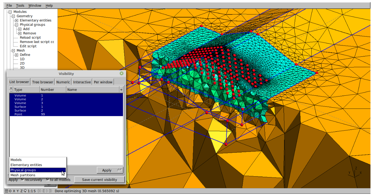
Gmsh visualization of the modelling mesh of the dike, with visibility dialog.#
Additional very useful material#
FreeCAD GeoMatics workbench (replaces GeoData workbench) allows for GPS, LiDAR and GIS data to be imported to FreeCAD