DC-EM joint inversion

Joint inversion is an important method to improve resolution properties by combining different methods. In the easiest case, the methods have the same subsurface parameter, for example direct current (DC) and electromagnetic (EM) measurements. In this example, we illustrate how two modelling operators can be combined by the JointInversion framework, using a vertical electric sounding (VES) and electromagnetic frequency sounding (FDEM).

A similar case has been documented by [Günther, 2013].

# We import the numpy and matplotlib
import numpy as np
import matplotlib.pyplot as plt
# Next we import pyGIMLi and the modelling operators for block models
import pygimli as pg
from pygimli.physics.em import HEMmodelling
from pygimli.physics.ves import VESModelling
from pygimli.frameworks import JointModelling
# For block models we need the Marquardt-Levenberg inversion scheme
from pygimli.frameworks import MarquardtInversion
from pygimli.viewer.mpl import drawModel1D

First we create a synthetic model and error models to be used later.

synThk = [5, 15, 15]
synRes = [1000, 100, 500, 20]
nlay = len(synRes)  # number of layers
errorEMabs = 1.  # absolute (ppm of primary signal)
errorDCrel = 3.  # in per cent
# we use the same starting model for all methods
startModel = [10]*(nlay-1) + [100]*nlay

Part 1: Electromagnetic sounding

We set forward operator and generate synthetic data with noise.

# MaxMin-10/Promys instrument, 1m above the ground
nf = 10
freq = 2**np.arange(nf) * 110.
fEM = HEMmodelling(nlay=nlay, height=1, f=freq, r=100, scaling="%")

dataEM = fEM(synThk + synRes)
errorEM = np.ones_like(dataEM) * errorEMabs
dataEM += pg.randn(len(dataEM), seed=1234) * errorEM

Result is inphase and outphase secondary fields divided by the primary field as a function of frequency. See inversion result & data fit figure below.

We first set up the independent EM inversion and run the model.

invEM = MarquardtInversion(fop=fEM, verbose=False)
modelEM = invEM.run(dataEM, np.abs(errorEM/dataEM), startModel=startModel)

Part 2: Vertical Electric Sounding

We set up the (DC) forward operator and generate synthetic data plus noise.

ab2 = 1.3**np.arange(20) * 3.  # logarithmically equidistance starting with 3m
na = len(ab2)
fDC = VESModelling(ab2=ab2, mn2=np.ones_like(ab2))
dataDC = fDC(synThk+synRes)
errorDC = np.ones_like(dataDC) * errorDCrel / 100.
dataDC *= 1. + pg.randn(len(dataDC), seed=1234) * errorDC

We set up the independent DC inversion and let it run.

invDC = MarquardtInversion(fop=fDC, verbose=False)
modelDC = invDC.run(dataDC, errorDC, startModel=startModel)

Part 3: Joint inversion

We create a the joint forward operator using the Joint inversion framework.

fDCEM = JointModelling([fDC, fEM])
fDCEM.setData([dataDC, dataEM])  # just for sizes!

Inversion is just as for the single inversions. The data vector is created by concatenating both data vectors. This is also done for the relative error.

jointData = pg.cat(dataDC, dataEM)
jointError = pg.cat(errorDC, np.abs(errorEM/dataEM))
invDCEM = MarquardtInversion(fop=fDCEM, verbose=False)
modelDCEM = invDCEM.run(jointData, jointError, startModel=startModel)

The final output of the inversion is plotted for every method. Most-important measure is the chi-squared misfit that should be close to 1.

for inv in [invEM, invDC, invDCEM]:
    inv.echoStatus()

print([invEM.chi2(), invDC.chi2(), invDCEM.chi2()])  # chi-square values

[1.0012335892601552, 1.1101824804524079, 1.0891389114139844]

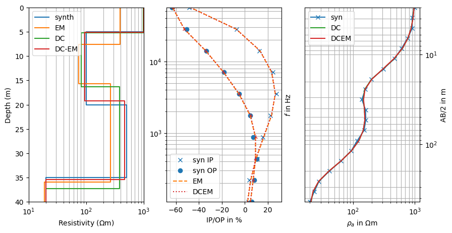
We finally plot the inverted models along with data and model responses.

fig, (ax1, ax2, ax3) = plt.subplots(figsize=(10, 5), ncols=3)
drawModel1D(ax1, synThk, synRes, plot='semilogx', color='C0', label="synth")
drawModel1D(ax1, model=modelEM, color='C1', label="EM")
drawModel1D(ax1, model=modelDC, color='C2', label="DC")
drawModel1D(ax1, model=modelDCEM, color='C3', label="DC-EM")
ax1.legend()
ax1.set_xlim((10., 1000.))
ax1.set_ylim((40., 0.))
ax1.grid(which='both')
ax2.semilogy(dataEM[0:nf], freq, 'x', color="C0", label='syn IP')
ax2.semilogy(dataEM[nf:nf*2], freq, 'o', color="C0", label='syn OP')
ax2.semilogy(invEM.response[0:nf], freq, '--', color="C1", label='EM')
ax2.semilogy(invEM.response[nf:nf*2], freq, '--', color="C1")
ax2.semilogy(invDCEM.response[na:na+nf], freq, ':', color="C3", label='DCEM')
ax2.semilogy(invDCEM.response[na+nf:na+nf*2], freq, '2:', color="C3")
ax2.set_ylim((min(freq), max(freq)))
ax2.set_xlabel("IP/OP in %")
ax2.set_ylabel("$f$ in Hz")
ax2.yaxis.set_label_position("right")
ax2.grid(which='both')
ax2.legend(loc="best")
ax3.loglog(dataDC, ab2, 'x-', label='syn', color="C0")
ax3.loglog(invDC.response, ab2, '-', label='DC', color="C2")
ax3.loglog(invDCEM.response[0:na], ab2, '-', label='DCEM', color="C3")
ax3.set_ylim((max(ab2), min(ab2)))
ax3.grid(which='both')
ax3.set_xlabel(r"$\rho_a$ in $\Omega$m")
ax3.set_ylabel("AB/2 in m")
ax3.yaxis.set_ticks_position("right")
ax3.yaxis.set_label_position("right")
ax3.legend()

<matplotlib.legend.Legend object at 0x7f7b68657d30>

All three inversions are able to reveal the subsurface structures. EM fails to describe the first layer-resistivity and also its thickness, for which DC does a better job. Both are similarly away from the synthetic model regarding the resistivity and upper depth of the third layer. EM can better resolve the good conductor at depth as expected. The joint inversion result combines the resolution properties of both methods and yields a result that is very close to the synthetic.

# Günther, T. (2013): On Inversion of Frequency Domain Electromagnetic Data in
# Salt Water Problems - Sensitivity and Resolution. Ext. Abstr., 19th European
# Meeting of Environmental and Engineering Geophysics, Bochum, Germany.