Note
Go to the end to download the full example code
Timelapse ERT#
Since pyGIMLi we have a class dedicated to timelapse ERT processing & inversion. The inversion supports different schemes from simple individual over constrained inversion to fully coupled (“4D”) inversion using pyGIMLi’s MultiFrameModelling modelling framework. Additionally, we created a github repository gimli-org/timelapseERT that holds published data and scripts demonstrating how to achieve the published results, according to the FAIR data standards.
This notebook is a simplistic model for a synthetic case.
We import the used libraries pygimli, meshtools the ERT module.
import numpy as np
import matplotlib.pyplot as plt
import pygimli as pg
import pygimli.meshtools as mt
from pygimli.physics import ert
We create a data container with a dipole-dipole array.
scheme = ert.createData(elecs=41, spacing=1, schemeName='dd', maxSeparation=15)
print(scheme)
Data: Sensors: 41 data: 465, nonzero entries: ['a', 'b', 'k', 'm', 'n', 'valid']
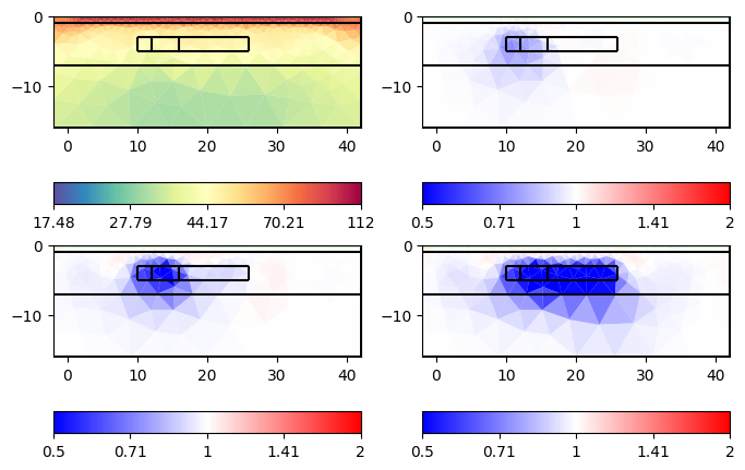
Our subsurface is a three-layer model with an aquifer in the middle, into which synthetic tracer is injected that is moving to the right.
world = mt.createWorld(start=[-50, 0], end=[100, -50], boundary=1,
                       layers=[-1, -7], worldMarker=True)
for pos in scheme.sensorPositions():
    world.createNode(pos, marker=-99)
    world.createNode(pos+pg.RVector3(0, -0.2))

# Create some heterogeneous block
plcs = [world]
pos = [10, 12, 16, 26]
nT = len(pos) - 1  # number of time steps
for i in range(nT):
    block = mt.createRectangle(start=[pos[i], -5], end=[pos[i+1], -3],
                               area=0.1, marker=4+i)
    plcs.append(block)

geom = mt.mergePLC(plcs)
mesh = mt.createMesh(geom, quality=34.4)
print(mesh)
ax, _ = pg.show(mesh, markers=True, boundaryMarkers=False, showMesh=True)
ax.set_xlim(0, 40)
ax.set_ylim(-10, 0)
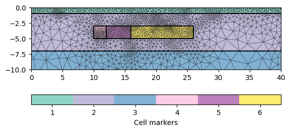
Mesh: Nodes: 2927 Cells: 5541 Boundaries: 8467

(-10.0, 0.0)
We associate 100 Ohmm to the first layer, 50 to the second and 20 to the last one. At the beginning, the anomalies have the same resistivity as the aquifer.
rhomap = [[1, 100.0], [2, 50.0], [3, 20.0], [4, 50.0], [5, 50.0], [6, 50.0]]
noise = dict(noiseLevel=0.01, noiseAbs=0, verbose=False)
mgr = ert.Manager()
data = ert.simulate(mesh=mesh, res=rhomap, scheme=scheme, **noise)
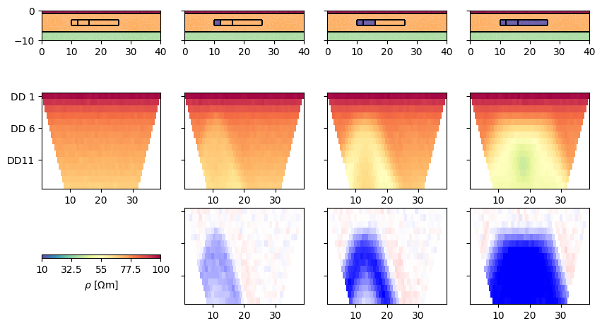
rhoTracer = 10
cDict = dict(colorBar=False, cMin=10, cMax=100, logScale=1, cMap='Spectral_r')
fig, ax = plt.subplots(figsize=(10, 6), ncols=nT+1, nrows=3)
DATA = []
for i in range(nT+1):
pg.show(mesh, rhomap, ax=ax[0, i], **cDict)
ax[0, i].set_xlim(0, 40)
ax[0, i].set_ylim(-10, 0)
data = ert.simulate(mesh, res=rhomap, scheme=scheme, **noise)
data.save('data{:d}.dat'.format(i))
DATA.append(data)
ert.show(data, ax=ax[1, i], **cDict)
ratio = data('rhoa') / DATA[0]('rhoa')
if i > 0:
ert.show(data, ratio, ax=ax[2, i],
cMap='bwr', cMin=1/1.5, cMax=1.5, colorBar=False)
if i < nT:
rhomap[3+i][1] = rhoTracer
for i in range(nT):
for j in range(3):
ax[j, i+1].set_yticklabels([])
cDict.pop('colorBar')
cDict['label'] = r'$\rho$ [$\Omega$m]'
pg.viewer.mpl.colorbar.createColorBarOnly(ax=ax[2, 0], **cDict)
ax[2, 0].set_aspect(3)
We initialize the TimelapseERT class by passing the list of data. Otherways are passing * a single data file that either holds all timestep or is accompagnied by another file with the apparent resistivites (and optionally errors) as matrix * a file name with a * in it that points to a number of data (e.g. bla*.dat) to be read sequentially Note that in the latter case or when passing a list of DataContainerERT the data will be homogenized, i.e. brought to a single DataContainerERT and a apparent resistivity matrix where non-existing values are masked out. In the initialization, one can pass a list of datatime objects to specify measuring times. Otherwise they are retrieved from the filenames or just set to equidistant intervals.
tl = ert.TimelapseERT(DATA)
print(tl)
Timelapse ERT data:
Data: Sensors: 41 data: 465, nonzero entries: ['a', 'b', 'k', 'm', 'n', 'valid']
4 time steps from 2023-10-27 13:46 to 2023-10-30 13:46
Masking of data can be achieved by tl.mask() specifying minimum and maximum apparent resistivity or maximum error. Additionally, you can filter the data by tl.filter() to set maximum geometric factor or remove/select timesteps. This command can generate multi-page pdfs of the data. tl.generateDataPDF(cMin=30, cMax=100)
One can do a single timestep inversion using tl.invert(t=i). If this argument is omitted, are timesteps are inverted sequentially, always using the ERT Manager. By default, the first model is used as reference, i.e. the model difference is constrained. This can be deactivatey by isReference=False. The reference model can be moved along with the inversion by by creep=True so that the difference to the preceding step is constrained. One can specify regularization options using a reg dictionary and, if wanted, a different regularization for the timesteps by regTL.
tl.invert(zWeight=0.3, lam=100)
print(tl.chi2s)
[0.21226409496298643, 0.1341141177729159, 0.14499314351159157, 0.4086383990426485]
After inversion, on can show the models by tl.showAllModels. For convenience (and if many timesteps are involved), one can also generate a multi-page pdf by tl.generateModelPDF. The user can access the individual models by tl.models[i] and plot them using tl.mgr.showResult(tl.models[i]) or pg.show(tl.pd, tl.models[i]).
tl.showAllModels();
for a in ax.flat:
    pg.viewer.mpl.drawPLC(a, geom, fillRegion=False, fitView=False)
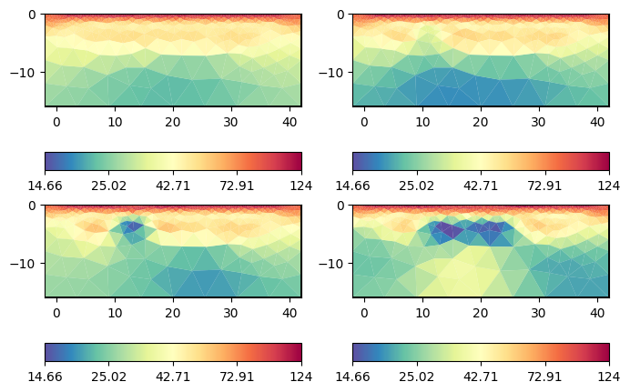
We can observe the major laying and also clear indications of the tracer injection. Often, one is interested in the changes or differences, which are in the usual logarithmic scale the ratios.
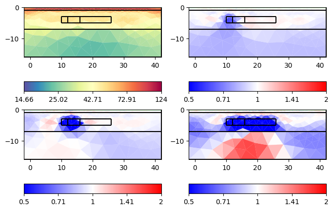
Here we see that we clearly see all the anomalies, but the first one is very slight due to its size. Additionally, we see artifacts of increased resistivity.
As powerful alternative to a sequential inversion, one can invert all timesteps together with constraints along the spatial and temporal dimensions. For this there is a special call fullInversion that might take more memory, but is usually not slower than a sequential inversion and moreover more robust.
708 model cells
Mesh: Nodes: 2030 Cells: 3820 Boundaries: 2984
fop: <pygimli.frameworks.timelapse.MultiFrameModelling object at 0x7fbe6a723100>
Data transformation: <pygimli.core._pygimli_.RTrans object at 0x7fbe6a8b2b00>
Model transformation: <pygimli.core._pygimli_.RTransLog object at 0x7fbe6a722930>
min/max (data): 22.64/100
min/max (error): 3%/3%
min/max (start model): 53.02/53.02
--------------------------------------------------------------------------------
inv.iter 0 ... chi² =  133.61
--------------------------------------------------------------------------------
inv.iter 1 ... chi² =    4.27 (dPhi = 94.12%) lam: 100.0
--------------------------------------------------------------------------------
inv.iter 2 ... chi² =    0.76 (dPhi = 54.55%) lam: 100.0


################################################################################
#                  Abort criterion reached: chi² <= 1 (0.76)                   #
################################################################################
Here, the results are gone due to the stabilizing smoothness across the time. To change the temporal smoothness, one can use the frame scale scalef, e.g., tl.fullInversion(scalef=0.5) for more changes in time.
References#
To be filled.
Total running time of the script: ( 0 minutes 35.450 seconds)