pygimli.physics.gravimetry

Solve gravimetric and magneto static problems in 2D and 3D analytically

Overview

Functions

BZPoly(pnts, poly, mag[, openPoly])	Vertical magnetic gradient for polygone.
BaZCylinderHoriz(pnts, R, pos, M)	Magnetic anomaly for a horizontal cylinder.
BaZSphere(pnts, R, pos, M)	Magnetic anomaly for a sphere.
SolveGravMagHolstein(*args, **kwargs)	Solve gravity and/or magnetics problem after Holstein (1997).
depthWeighting(mesh[, z0, height, power, ...])	Return Li&Oldenburg like depth weighting of boundaries or cells.
gradGZCylinderHoriz(r, a, rho[, pos])	TODO WRITEME.
gradGZHalfPlateHoriz(pnts, t, rho[, pos])	TODO WRITEME.
gradGZSphere(r, rad, rho[, pos])	TODO WRITEME.
gradUCylinderHoriz(r, a, rho[, pos])	2D Gradient of gravimetric potential of horizontal cylinder.
gradUHalfPlateHoriz(pnts, t, rho[, pos])	Gravitational field od a horizontal half plate.
gradUSphere(r, rad, rho[, pos])	Gravitational field of a sphere.
magneticDipole(Q, M[, P, x, y, z, alpha, ...])	Compute magnetic field according to eq.
solveGravimetry(mesh[, dDensity, pnts, complete])	Solve gravimetric response.
uCylinderHoriz(pnts, rad, rho[, pos])	Gravitational potential of horizonzal cylinder.
uSphere(r, rad, rho[, pos])	Gravitational potential of a sphere.

Classes

GravityModelling(mesh, points[, cmp])	Magnetics modelling operator using Holstein (2007).
GravityModelling2D([points])	Gravimetry modelling operator.
MagManager([data])	Magnetics Manager.
MagneticsModelling([mesh, points, cmp, ...])	Magnetics modelling operator using Holstein (2007).
RemanentMagneticsModelling(mesh, points[, ...])	Remanent magnetics modelling operator for arbitrary magnetization.

Functions

pygimli.physics.gravimetry.BZPoly(pnts, poly, mag, openPoly=False)

Vertical magnetic gradient for polygone.

Parameters:

• pnts (list) – Measurement points [[p1x, p1z], [p2x, p2z],…]

• poly (list) – Polygon [[p1x, p1z], [p2x, p2z],…]

• mag ([M_x, M_y, M_z]) – Magnetization = [M_x, M_y, M_z]

pygimli.physics.gravimetry.BaZCylinderHoriz(pnts, R, pos, M)

Magnetic anomaly for a horizontal cylinder.

Calculate the vertical component of the anomalous magnetic field Bz for a buried horizontal cylinder at position pos with radius R for a given magnetization M at measurement points pnts.

TODO .. only 2D atm

Parameters:

• pnts ([[x,z], ]) – measurement points – array[x,y,z]

• R (float) – radius

• pos ([float, float]) – [x,z] – sphere center

• M ([float, float]) – [Mx, Mz] – magnetization

pygimli.physics.gravimetry.BaZSphere(pnts, R, pos, M)

Magnetic anomaly for a sphere.

Calculate the vertical component of the anomalous magnetic field Bz for a buried sphere at position pos with radius R for a given magnetization M at measurement points pnts.

Parameters:

• pnts ([[x,y,z], ]) – measurement points – array[x,y,z]

• R (float) – radius

• pos ([float, float, float]) – [x,y,z] – sphere center

• M ([float, float, float]) – [Mx, My, Mz] – magnetization

pygimli.physics.gravimetry.SolveGravMagHolstein(*args, **kwargs)

Solve gravity and/or magnetics problem after Holstein (1997).

Parameters:

• mesh (pygimli:mesh) – tetrahedral or hexahedral mesh

• pnts (list|array of (x, y, z)) – measuring points

• cmp (list of str) – component list of type str, valid values are: gx, gy, gz, TFA, Bx, By, Bz, Bxx, Bxy, Bxz, Byy, Byz, Bzz

• igrf (list|array of size 3 or 7) –

  international geomagnetic reference field, either [D, I, H, X, Y, Z, F] - declination, inclination, horizontal field,

  X/Y/Z components, total field OR

  [X, Y, Z] - X/Y/Z components

Returns:

out – kernel matrix to be multiplied with density or susceptibility

Return type:

ndarray (nPoints x nComponents x nCells)

pygimli.physics.gravimetry.depthWeighting(mesh, z0: float = 25, height: float = 0, power: float = 1.5, normalize: bool = False, cell: bool = False)

Return Li&Oldenburg like depth weighting of boundaries or cells.

To account for inherent ambiguity in potential field methods, a depth weighting of the regulariation term is often applied in inversion, going back to Li & Oldenburg (1996, eq. 18):

\[w(z) = \frac{1}{(z+z_0)^{3/2}}\]

Here, we reformulate the original equation in order to make it unitless:

\[w(z) = \frac{1}{(z/z_0+1)^p}\]

Which is the same as before except a factor that can go into the regularization strength. The function describes a decay with depth, starting from w(0)=1 and approaching w(z)=0 for z>>z0. z is the depth of a boundary or cell below the sensor and is determined by its mesh center and the sensor position.

Parameters:

• z0 (float [25]) – centroid depth (w(z0)=1/2^p)

• height (float) – sensor height to be added to depth

• power (float [1.5]) – exponent

• normalize (bool [False]) – normalize such that the mean weight is 1 (like unweighted)

• cell (bool [True]) – use cell center (for cType=0|2|geostat) instead of boundary (cType=1)

Return type:

depth weighting vector for all interior boundaries or all cells

pygimli.physics.gravimetry.gradGZCylinderHoriz(r, a, rho, pos=(0.0, 0.0))

TODO WRITEME.

\[g = -grad u(r), with r = [x,z], |r| = \sqrt{x^2+z^2}\]

Parameters:

• r (list[[x, z]]) – Observation positions

• a (float) – Cylinder radius in [meter]

• rho – Density in [kg/m^3]

Return type:

grad gz, [gz_x, gz_z]

Examples using pygimli.physics.gravimetry.gradGZCylinderHoriz

Semianalytical Gravimetry and Geomagnetics in 2D

Semianalytical Gravimetry and Geomagnetics in 2D

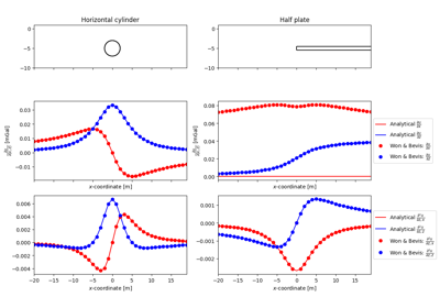
pygimli.physics.gravimetry.gradGZHalfPlateHoriz(pnts, t, rho, pos=(0.0, 0.0))

TODO WRITEME.

\[g = -\nabla u\]

Parameters:

• pnts (array (\(n\times 2\))) – n 2 dimensional measurement points

• t (float) – Plate thickness in \([\text{m}]\)

• rho (float) – Density in \([\text{kg}/\text{m}^3]\)

Returns:

gz – Gradient of z-component of g \(\nabla(\frac{\partial u}{\partial\vec{r}}_z)\)

Return type:

array

Examples using pygimli.physics.gravimetry.gradGZHalfPlateHoriz

Semianalytical Gravimetry and Geomagnetics in 2D

Semianalytical Gravimetry and Geomagnetics in 2D

pygimli.physics.gravimetry.gradGZSphere(r, rad, rho, pos=(0.0, 0.0, 0.0))

TODO WRITEME.

\[g = -\nabla u\]

Parameters:

• r ([float, float, float]) – position vector

• rad (float) – radius of the sphere

• rho (float) – density in [kg/m^3]

Return type:

[d g_z /dx, d g_z /dy, d g_z /dz]

pygimli.physics.gravimetry.gradUCylinderHoriz(r, a, rho, pos=(0.0, 0.0))

2D Gradient of gravimetric potential of horizontal cylinder.

\[g = -G[m^3/(kg s^2)] * dM[kg/m] * 1/r[1/m] * grad(r)[1/1] = [m^3/(kg s^2)] * [kg/m] * 1/m * [1/1] == m/s^2\]

Parameters:

• r (list[[x, z]]) – Observation positions

• a (float) – Cylinder radius in [meter]

• pos ([x,z]) – Center position of cylinder.

• rho (float) – Delta density in [kg/m^3]

Returns:

g – Gradient of gravimetry potential [mGal].

Return type:

[dudx, dudz]

Examples using pygimli.physics.gravimetry.gradUCylinderHoriz

Semianalytical Gravimetry and Geomagnetics in 2D

Semianalytical Gravimetry and Geomagnetics in 2D

Gravimetry in 2D - Part I

Gravimetry in 2D - Part I

pygimli.physics.gravimetry.gradUHalfPlateHoriz(pnts, t, rho, pos=(0.0, 0.0))

Gravitational field od a horizontal half plate.

\[g = -grad u,\]

Parameters:

• pnts

• t

• rho – Density in [kg/m^3]

Returns:

z-component of g .. math:: nabla(partial u/partialvec{r})_z

Return type:

gz

Examples using pygimli.physics.gravimetry.gradUHalfPlateHoriz

Semianalytical Gravimetry and Geomagnetics in 2D

Semianalytical Gravimetry and Geomagnetics in 2D

pygimli.physics.gravimetry.gradUSphere(r, rad, rho, pos=(0.0, 0.0, 0.0))

Gravitational field of a sphere.

\[g = -G[m^3/(kg s^2)] * dM[kg] * 1/r^2 1/m^2] * \grad(r)[1/1] = [m^3/(kg s^2)] * [kg] * 1/m^2 * [1/1] == m/s^2\]

Parameters:

• r ([float, float, float]) – position vector

• rad (float) – radius of the sphere

• rho (float) – density in [kg/m^3]

Returns:

[gx, gy, gz] – gravitational acceleration (note that gz points negative)

Return type:

[float*3]

pygimli.physics.gravimetry.magneticDipole(Q, M, P=None, x=None, y=0.0, z=0.0, alpha: float = 0, cylinder: bool = False)

Compute magnetic field according to eq. (4.14) from Blakely (1996).

The magnetic field \(\vec{B}\) at a point P due to a dipole in Q reads

\[\vec{B}(\vec{r}) = \frac{\mu_0 M}{4\pi r^3} \left[ 3 (\vec{M}' \cdot \vec{r}')\vec{r}' - \vex{M}' \right]\]

where \(\vec r=\vec r_P - \vec r_Q\) is the vector between the magnetic moment Q and the measuring point P, \(r'/M'\) are unit vectors of r/M.

Parameters:

• Q (array 3x1) – position of magnetic dipole

• M (array 3x1) – magnetization vector

• P (array 3xN) – measuring positions

• x (array N) – positions as profile

• y/z (array | float) – y and z positions

• alpha (profile direction (degree)) – profile direction

• cylinder (bool [False]) – use line/cylinder instead of point/sphere

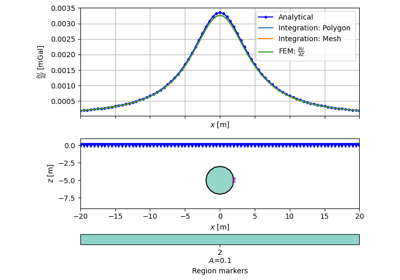
pygimli.physics.gravimetry.solveGravimetry(mesh, dDensity=None, pnts=None, complete=False)

Solve gravimetric response.

2D with pygimli.physics.gravimetry.lineIntegralZ_WonBevis

3D with pygimli.physics.gravimetry.gravMagBoundarySinghGup

Parameters:

• mesh (GIMLI::Mesh) – 2d or 3d mesh with or without cells.

• dDensity (float | array) –

  Density difference.

  • float – solve for positive boundary marker only.

    Assuming one inhomogeneity.

  • [[int, float]] – solve for multiple positive boundaries TOIMPL

  • array – solve for one delta density value per cell

  • None – return per cell kernel matrix G TOIMPL

• pnts ([[x_i, y_i]]) – List of measurement positions.

• complete (bool [False]) – If True return whole solution or matrix for [dgx, dgy, dgz]

Returns:

• dg (array OR)

• dz, dgz (arrays (if complete))

Examples using pygimli.physics.gravimetry.solveGravimetry

Semianalytical Gravimetry and Geomagnetics in 2D

Semianalytical Gravimetry and Geomagnetics in 2D

Gravimetry in 2D - Part I

Gravimetry in 2D - Part I

pygimli.physics.gravimetry.uCylinderHoriz(pnts, rad, rho, pos=None)

Gravitational potential of horizonzal cylinder.

Parameters:

• pnts (iterable) – measuring point locations

• rad (float) – radius of the cylinder

• rho (float) – density contrast in kg/m^3

• pos ([float, float]) – x,z position of the cylinder axis

Return type:

gravimetric potential at the given points

pygimli.physics.gravimetry.uSphere(r, rad, rho, pos=None)

Gravitational potential of a sphere.

Gravitational potential of a sphere with radius and density at a given position.

\[u = -G * dM * \frac{1}{r}\]

Parameters:

• r ([float, float, float]) – position vector

• rad (float) – radius of the sphere

• rho (float) – density

• pos ([float, float, float]) – position of sphere (0.0, 0.0, 0.0)

Classes

class pygimli.physics.gravimetry.GravityModelling(mesh, points, cmp=None)

Bases: MeshModelling

Magnetics modelling operator using Holstein (2007).

__init__(mesh, points, cmp=None)

Set up forward operator.

Parameters:

• mesh (pygimli:mesh) – tetrahedral or hexahedral mesh

• points (list|array of (x, y, z)) – measuring points

• cmp (list of str) – component of: gx, gy, gz

createJacobian(model)

Do nothing as this is a linear problem.

createKernel()

Create computational kernel.

response(model)

Compute forward response.

setMesh(mesh, ignoreRegionManager=False)

Set the mesh.

class pygimli.physics.gravimetry.GravityModelling2D(points=None, **kwargs)

Bases: MeshModelling

Gravimetry modelling operator.

__init__(points=None, **kwargs)

Initialize forward operator, optional with mesh and points.

You can specify both the mesh and the measuring points, or set the latter after the mesh has been set.

Parameters:

• mesh (pg.Mesh) – mesh for forward computation

• points (array[x,y]) – measuring points

calcMatrix()

Create Jacobian matrix (density-independent).

createJacobian(model)

Create Jacobian.

createStartmodel(*args)

Create the default starting model.

response(model)

Calculate response for a given density distribution.

setSensorPositions(pnts)

Set measurement locations. [[x,y,z],…].

class pygimli.physics.gravimetry.MagManager(data=None, **kwargs)

Bases: MeshMethodManager

Magnetics Manager.

__init__(data=None, **kwargs)

Create Magnetics Manager instance.

createForwardOperator(verbose=False)

Create forward operator (computationally extensive!).

createGrid(dx: float = 50, depth: float = 800, bnd: float = 0)

Create a grid.

Parameters:

• dx (float=50) – Grid spacing in x and y direction.

• depth (float=800) – Depth of the grid in z direction.

• bnd (float=0) – Boundary distance to extend the grid in x and y direction.

Returns:

mesh – Created 3D structured grid.

Return type:

GIMLI::Mesh

createMesh(boundary: float = 0, area: float = 100000.0, depth: float = 0, quality: float = 1.3, addPLC: Mesh = None, addPoints: bool = True, frame: float = 0)

Create an unstructured 3D mesh.

Parameters:

• boundary (float=0) – Boundary distance to extend the mesh in x and y direction.

• area (float=1e5) – Maximum area constraint for cells.

• depth (float=0) – Depth of the mesh in z direction.

• quality (float=1.3) – Quality factor for mesh generation.

• addPLC (GIMLI::Mesh) – PLC mesh to add to the mesh.

• addPoints (bool=True) – Add points from self.x and self.y to the mesh.

Returns:

mesh – Created 3D unstructured mesh.

Return type:

GIMLI::Mesh

createMeshOld(bnd: float = 0, area: float = 100000.0, depth: float = 0, quality: float = 1.3, addPLC: Mesh = None, addPoints: bool = True)

Create an unstructured 3D mesh.

Parameters:

• bnd (float=0) – Boundary distance to extend the mesh in x and y direction.

• area (float=1e5) – Maximum area constraint for cells.

• depth (float=0) – Depth of the mesh in z direction.

• quality (float=1.3) – Quality factor for mesh generation.

• addPLC (GIMLI::Mesh) – PLC mesh to add to the mesh.

• addPoints (bool=True) – Add points from self.x and self.y to the mesh.

Returns:

mesh – Created 3D unstructured mesh.

Return type:

GIMLI::Mesh

detectLines(**kwargs)

Detect lines in data.

Keyword Arguments:

• mode (str|float|array) – ‘x’/’y’: along coordinate axis spacing vector: by given spacing float: minimum distance

• axis (str='x') – Axis to use for line detection.

• show (bool=False) – Show detected lines.

inversion(noise_level=2, noisify=False, **kwargs)

Run Inversion (requires mesh and FOP).

Parameters:

• noise_level (float|array) – absolute noise level (absoluteError)

• noisify (bool) – add noise before inversion

• relativeError (float|array [0.01]) – relative error to stabilize very low data

• depthWeighting (bool [True]) – apply depth weighting after Li&Oldenburg (1996)

• z0 (float) – skin depth for depth weighting

• mul (array) – multiply constraint weight with

Keyword Arguments:

• startModel (float|array=0.001) – Starting model (typically homogeneous)

• relativeError (float=0.001) – Relative error to stabilize very low data.

• lam (float=10) – regularization strength

• verbose (bool=True) – Be verbose

• symlogThreshold (float [0]) – Threshold for symlog data trans.

• limits ([float, float]) – Lower and upper parameter limits.

• C (int|Matrix|[float, float, float] [1]) – Constraint order.

• C(,cType) (int|Matrix|[float, float, float]=C) – Constraint order, matrix or correlation lengths.

• z0 (float=25) – Skin depth for depth weighting.

• depthWeighting (bool=True) – Apply depth weighting after Li&Oldenburg (1996).

• mul (float=1) – Multiply depth weighting constraint weight with this factor.

• **kwargs – Additional keyword arguments for the inversion.

Returns:

model – Model vector (also saved in self.inv.model).

Return type:

np.array

loadResults(folder)

Load inversion results from a folder.

Parameters:

folder (str) – Folder to load results from.

saveResults(folder=None)

Save inversion results to a folder.

Parameters:

folder (str) – Folder to save results to.

setMesh(mesh)

Set or load mesh.

show3DModel(label: str = None, trsh: float = 0.025, synth: Mesh = None, invert: bool = False, position: str = 'yz', elevation: float = 10, azimuth: float = 25, zoom: float = 1.2, **kwargs)

Show standard 3D view.

Parameters:

• label (str='sus') – Label for the mesh data to visualize.

• trsh (float=0.025) – Threshold for the mesh data to visualize.

• synth (GIMLI::Mesh [None]) – Synthetic model to visualize in wireframe.

• invert (bool=False) – Invert the threshold filter.

• position (str="yz") – Camera position, e.g., “yz”, “xz”, “xy”.

• elevation (float=10) – Camera elevation angle.

• azimuth (float=25) – Camera azimuth angle.

• zoom (float=1.2) – Camera zoom factor.

Keyword Arguments:

• cMin (float=0.001) – Minimum color value for the mesh data.

• cMax (float=None) – Maximum color value for the mesh data. If None, it is set to the maximum value of the mesh data.

• cMap (str="Spectral_r") – Colormap for the mesh data visualization.

• logScale (bool=False) – Use logarithmic scale for the mesh data visualization.

• kwargs – Additional keyword arguments for the pyvista plot.

Returns:

pl – Plot widget with the 3D model visualization.

Return type:

pyvista Plotter

showData(cmp=None, **kwargs)

Show data.

showDataFit(**kwargs)

Show data, model response and misfit.

Keyword Arguments:

• cmap (str ['bwr']) – colormap

• maxField (float) – colorbar for field

• maxMisfit (float) – colorbar for (error-weighted) misfit

• vmin/vmax (float) – colorbar limits

showLineData(line=None, cmp=None, **kwargs)

Show data for a specific line.

Parameters:

• line (int|array) – Line number or array of line numbers to show.

• cmp (list) – List of components to show.

class pygimli.physics.gravimetry.MagneticsModelling(mesh=None, points=None, cmp=None, igrf=None, verbose=False)

Bases: MeshModelling

Magnetics modelling operator using Holstein (2007).

__init__(mesh=None, points=None, cmp=None, igrf=None, verbose=False)

Set up forward operator.

Parameters:

• mesh (pygimli:mesh) – Tetrahedral or hexahedral mesh.

• points (list|array of (x, y, z)) – Measuring points.

• cmp ([str,]) – Component of: gx, gy, gz, TFA, Bx, By, Bz, Bxy, Bxz, Byy, Byz, Bzz

• igrf (list|array of size 3 or 7) –

  International geomagnetic reference field. either:

  • [D, I, H, X, Y, Z, F] - declination,

    inclination, horizontal field, X/Y/Z components, total field OR

  • [X, Y, Z] - X/Y/Z

    components OR

  • [lat, lon] - latitude,

    longitude (automatic by pyIGRF)

computeKernel()

Compute the kernel.

createJacobian(model)

Do nothing as this is a linear problem.

Abstract method to create the Jacobian matrix. Need to be implemented in derived classes.

Parameters:

model (array-like) – Model parameters.

response(model)

Compute forward response.

Parameters:

model (array-like) – Model parameters.

class pygimli.physics.gravimetry.RemanentMagneticsModelling(mesh, points, cmp=None, igrf=None)

Bases: MagneticsModelling

Remanent magnetics modelling operator for arbitrary magnetization.

__init__(mesh, points, cmp=None, igrf=None)

Set up forward operator.

Parameters:

• mesh (pygimli:mesh) – Tetrahedral or hexahedral mesh.

• points (list|array of (x, y, z)) – Measuring points.

• cmp ([str,]) – Component of: gx, gy, gz, TFA, Bx, By, Bz, Bxy, Bxz, Byy, Byz, Bzz

• igrf (list|array of size 3 or 7) –

  International geomagnetic reference field. either:

  • [D, I, H, X, Y, Z, F] - declination,

    inclination, horizontal field, X/Y/Z components, total field OR

  • [X, Y, Z] - X/Y/Z

    components OR

  • [lat, lon] - latitude,

    longitude (automatic by pyIGRF)

createJacobian(model)

Do nothing.

response(model)

Add together all three responses.