Basics of Finite Element Analysis

This tutorial covers the first steps into Finite Element computation referring the M (Modelling) in pyGIMLi.

We will not dig into deep details about the theory of the Finite Elements Analysis (FEA) here, as this can be found in several books, e.g., [Zienkiewicz, 1977].

Anyhow, there is a little need for theory to understand what it means to use FEA for the solution of a boundary value problem. So we start with some basics.

Assuming Poisson’s equation as a simple partial differential problem to be solved for the sought scalar field \(u(\mathbf{r})\) within a modelling domain \(\mathbf{r}\in\Omega\) with a non zero right hand side function \(f\).

\[\begin{split}- \Delta u & = f \quad{\mathrm{in}}\quad~\Omega\\ u & = g \quad{\mathrm{on}}\quad\partial\Omega\;.\end{split}\]

The Laplace operator \(\Delta = \nabla\cdot\nabla\) given by the divergence of the gradient, is the sum of the second partial derivatives of the field \(u(\mathbf{r})\) with respect to the Cartesian coordinates in 1D space \(\mathbf{r} = (x)\), in 2D \(\mathbf{r} = (x, y)\), or 3D space \(\mathbf{r} = (x, y, z)\). On the boundary \(\partial\Omega\) of the domain, we want known values of \(u=g\) as so called Dirichlet boundary conditions.

A common approach to solve this problem is the method of weighted residuals. The base assumption states that an approximated solution \(u_h\approx u\) will only satisfy the differential equation with a rest \(R\): \(\Delta u_h + f = R\). If we choose some weighting functions \(w\), we can try to minimize the resulting residuum over our modelling domain as:

\[\int_{\Omega} R w = 0\;,\]

which leads to:

\[\int_{\Omega} - \Delta u_h w = \int_{\Omega} f w\;.\]

It is preferable to eliminate the second derivative in the Laplace operator, either due to integration by parts or by applying the product rule and Gauss’s law. This leads to the so called weak formulation:

\[\begin{split}\int_{\Omega} \nabla u_h \nabla w - \int_{\partial \Omega}\mathbf{n}\nabla u_h w & = \int_{\Omega} f w \\ \int_{\Omega} \nabla u_h \nabla w & = \int_{\Omega} f w + \int_{\partial \Omega}\frac{\partial u_h}{\partial\mathbf{n}} w\;.\end{split}\]

We can solve these integrals after choosing an appropriate basis for an approximate solution \(u_h\) as:

\[u_h = \sum_i \mathrm{u}_i N_i\quad\text{with}\quad i = 0\ldots\mathcal{N}\;.\]

The latter fundamental FEA relation discretizes the continuous solution \(u_h\) into a discrete values \(\mathrm{u} = \{\mathrm{u}_i\}\) for a number of \(i = 0\ldots\mathcal{N}\) discrete points, usually called nodes.

The basis functions \(N_i\) can be understood as interpolation rules for the discrete solution between adjacent nodes and will be chosen later.

Now we can set the unknown weighting functions to be the same as the basis functions \(w=N_j\) with \(j=0\ldots\mathcal{N}\) (Galerkin method)

\[\begin{split}\int_{\Omega} \sum_i \mathrm{u}_i \nabla N_i \nabla N_j\\ & = \int_{\Omega} f_j N_j + \int_{\partial \Omega} h N_j \quad \text{with}\quad h\\ & = \frac{\partial u}{\partial \mathbf{n}}\end{split}\]

this can be rewritten with \(h=0\) as:

\[\begin{split}\mathrm{A} \mathrm{u} &= \mathrm{b} \\ & \text{with} \\ \mathrm{A} & = \{\mathrm{a}_{i,j}\} = \int_{\Omega}\nabla N_i \nabla N_j \quad\text{known as 'Stiffness matrix'}\\ \mathrm{b} & = \{\mathrm{b}_j\} = \int_{\Omega} f_j N_j \quad\text{known as 'Load vector'}\end{split}\]

The solution of this linear system of equations leads to the discrete solution \(\mathrm{u} = \{\mathrm{u}_i\}\) for all \(i=1\ldots\mathcal{N}\) nodes inside the modelling domain.

For the practical part, the choice of the nodes is crucial. If we choose too little, the accuracy of the sought solution might be too small. If we choose too many, the dimension of the system matrix will be too large, which leads to higher memory consumption and calculation times.

To define the nodes, we discretize our modelling domain into cells, or the eponymous elements. Cells are basic geometric shapes like triangles or hexahedrons and are constructed from the nodes and collected in a mesh. See the tutorials about the mesh basics (Basics). In summary, the discrete solutions of the differential equation using FEA on a specific mesh are defined on the node positions of the mesh.

The chosen mesh cells also define the base functions and the integration rules that are necessary to assemble the stiffness matrix and the load vector and will be discussed in a different tutorial (TOWRITE link here).

To finally solve our little example we still need to handle the application of the boundary condition \(u=g\) which is called Dirichlet condition. Setting explicit values for our solution is not covered by the general Galerkin weighted residuum method but we can solve it algebraically. We reduce the linear system of equations by the known solutions \(g={g_k}\) for all \(k\) nodes on the affected boundary elements: (maybe move this to the BC tutorial)

\[\begin{split}\mathrm{A_D}\cdot\mathrm{u} &= \mathrm{b_D} \\ & \text{with} \\ \mathrm{A_D} & = \{\mathrm{a}_{i,j}\}\quad\forall i, j ~\notin~ k ~\text{and}~1~\text{for}~i,j \in k\\ \mathrm{b_D} & = \{\mathrm{b}_j\} - \mathrm{A}\cdot\mathrm{g}\quad\forall j \notin k~\text{and}~g_k~\text{for}~j \in k\end{split}\]

Now we have all parts together to assemble \(\mathrm{A_D}\) and \(\mathrm{b_D}\) and finally solve the given boundary value problem.

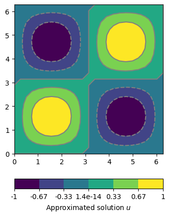
It is usually a good idea to test a numerical approach with known solutions. To keep things simple we create a modelling problem from the reverse direction. We choose a solution, calculate the right hand side function and select the domain geometry suitable for nice Dirichlet values.

\[\begin{split}u(x,y) & = \operatorname{sin}(x)\operatorname{sin}(y)\\ - \Delta u & = f(x,y) = 2 \operatorname{sin}(x)\operatorname{sin}(y)\\ \Omega \in I\!R^2 & \quad \text{on}\quad 0 \leq x \leq 2\pi,~~ 0 \leq y \leq 2\pi \\ u & = g = 0 \quad \text{on}\quad \partial \Omega\end{split}\]

We now can solve the Poison equation applying the FEA capabilities of pygimli and compare the resulting approximate solution \(\mathrm{u}\) with our known exact solution \(u(x,y)\).

import numpy as np
import pygimli as pg

We start to define the modelling domain and functions for the exact solution and the values for the load vector. The desired mesh of our domain will be a grid with equidistant spacing in x and y directions.

domain = pg.createGrid(x=np.linspace(0.0, 2*np.pi, 25),
                       y=np.linspace(0.0, 2*np.pi, 25))

uExact = lambda pos: np.sin(pos[0]) * np.sin(pos[1])
f = lambda cell: 2.0 * np.sin(cell.center()[0]) * np.sin(cell.center()[1])

We use the existing shortcut functions for the assembling of the basic FEA system matrices and vectors. The implemented parts of the solving process are supposed to be dimension independent. You only need to find a valid mesh with the supported element types.

A = pg.solver.createStiffnessMatrix(domain)
b = pg.solver.createLoadVector(domain, f)

To apply the boundary condition we first need to identify all boundary elements. The default grid applies the following boundary marker on the outermost boundaries: 1 (left), 2(right), 3(top), and 4(bottom).

boundaries = pg.solver.parseArgToBoundaries({'1,2,3,4': 0.0}, domain)

parseArgToBoundaries is a helper function to collect a list of tupels (Boundary element, value), which can be used to apply the Dirichlet conditions.

pg.solver.assembleDirichletBC(A, boundaries, b)

{25: 0.0, 0: 0.0, 50: 0.0, 75: 0.0, 100: 0.0, 125: 0.0, 150: 0.0, 175: 0.0, 200: 0.0, 225: 0.0, 250: 0.0, 275: 0.0, 300: 0.0, 325: 0.0, 350: 0.0, 375: 0.0, 400: 0.0, 425: 0.0, 450: 0.0, 475: 0.0, 500: 0.0, 525: 0.0, 550: 0.0, 575: 0.0, 600: 0.0, 24: 0.0, 49: 0.0, 74: 0.0, 99: 0.0, 124: 0.0, 149: 0.0, 174: 0.0, 199: 0.0, 224: 0.0, 249: 0.0, 274: 0.0, 299: 0.0, 324: 0.0, 349: 0.0, 374: 0.0, 399: 0.0, 424: 0.0, 449: 0.0, 474: 0.0, 499: 0.0, 524: 0.0, 549: 0.0, 574: 0.0, 599: 0.0, 624: 0.0, 1: 0.0, 2: 0.0, 3: 0.0, 4: 0.0, 5: 0.0, 6: 0.0, 7: 0.0, 8: 0.0, 9: 0.0, 10: 0.0, 11: 0.0, 12: 0.0, 13: 0.0, 14: 0.0, 15: 0.0, 16: 0.0, 17: 0.0, 18: 0.0, 19: 0.0, 20: 0.0, 21: 0.0, 22: 0.0, 23: 0.0, 601: 0.0, 602: 0.0, 603: 0.0, 604: 0.0, 605: 0.0, 606: 0.0, 607: 0.0, 608: 0.0, 609: 0.0, 610: 0.0, 611: 0.0, 612: 0.0, 613: 0.0, 614: 0.0, 615: 0.0, 616: 0.0, 617: 0.0, 618: 0.0, 619: 0.0, 620: 0.0, 621: 0.0, 622: 0.0, 623: 0.0}

The approximate solution \(\mathrm{u}\) can then be found as the solution of the linear system of equations.

u = pg.solver.linSolve(A, b)

The resulting scalar field can displayed with the pg.show shortcut.

ax, cb = pg.show(domain, u, label='Approximated solution $u$', nLevs=7)

For analyzing the accuracy for the approximation we apply the L2 norm for the finite element space pygimli.solver.normL2 for a set of different solutions with decreasing cell size. Instead of using the the single assembling steps again, we apply our Finite Element shortcut function pygimli.solver.solve.

domain = pg.createGrid(x=np.linspace(0.0, 2*np.pi, 3),
                       y=np.linspace(0.0, 2*np.pi, 3))

h = []
l2 = []
for i in range(5):
    domain = domain.createH2()
    u_h = pg.solve(domain, f=f, bc={'Dirichlet':{'1:5': 0}})
    u = np.array([uExact(_) for _ in domain.positions()])
    l2.append(pg.solver.normL2(u - u_h, domain))
    h.append(min(domain.boundarySizes()))
    print("NodeCount: {0}, h:{1}m, L2:{2}%".format(domain.nodeCount(),
                                                   h[-1], l2[-1]))

ax,_ = pg.show()
ax.loglog(h, l2, 'o-')
ax.set_ylabel('Approximation error: $L_2$ norm')
ax.set_xlabel('Cell size $h$ (m)')
ax.grid()

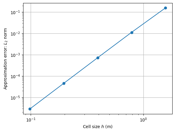
NodeCount: 25, h:1.5707963267948966m, L2:0.15650280987445644%
NodeCount: 81, h:0.7853981633974474m, L2:0.011159591448055969%
NodeCount: 289, h:0.3926990816987228m, L2:0.0007191303723399217%
NodeCount: 1089, h:0.1963495408493614m, L2:4.52847247960416e-05%
NodeCount: 4225, h:0.09817477042467981m, L2:2.835595560299441e-06%

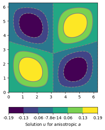
We calculated the examples before for a homogeneous material parameter a=1, but we can apply any heterogeneous values to0. One way is to create a list of parameter values, one for each cell of the domain. Currently the values for each cell can be of type float, complex, or real valued anisotropy or constitutive matrix. For illustration we show a calculation with an anisotropic material. We simply use the same setting as above and assume a -45 degree dipping angle in the left and 45 degree dipping in the right part of the domain. Maybe we will find someday a more meaningful example. If you have an idea please don’t hesitate to share.

a = [None]*domain.cellCount()
for c in domain.cells():
    if c.center()[0] < np.pi:
        a[c.id()] = pg.solver.createAnisotropyMatrix(lon=1.0, trans=10.0,
                                               theta=-45/180 * np.pi)
    else:
        a[c.id()] = pg.solver.createAnisotropyMatrix(lon=1.0, trans=10.0,
                                               theta=45/180 * np.pi)

u = pg.solve(domain, a=a, f=f, bc={'Dirichlet':{'*': 0}})
ax, cb = pg.show(domain, u, label='Solution $u$ for anisotropic $a$', nLevs=7)