ERT field data with topography

Simple example of data measured over a slagdump demonstrating:

• 2D inversion with topography

• geometric factor generation

• topography effect

import pygimli as pg
from pygimli.physics import ert

Get some example data with, typically by a call like data = ert.load(“filename.dat”) that supports various file formats

data = pg.getExampleData('ert/slagdump.ohm', verbose=True)
print(data)

[:::::::::::::::::::::::::::::::::::: 100% ::::::::::::::::::::::::::::::::::::] 5435 of 5435 complete
md5: f27293809709e8fdc89bfb0a55e6e1ec
Data: Sensors: 38 data: 222, nonzero entries: ['a', 'b', 'm', 'n', 'r', 'valid']

The data file does not contain geometric factors (token field ‘k’), so we create them based on the given topography.

data['k'] = ert.createGeometricFactors(data, numerical=True)

We initialize the ERTManager for further steps and eventually inversion.

mgr = ert.ERTManager(sr=False)

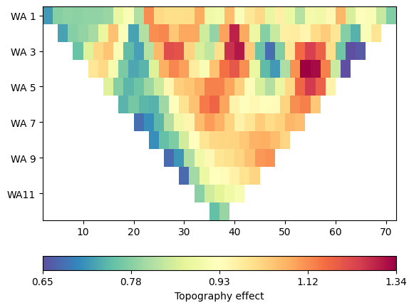
It might be interesting to see the topography effect, i.e the ratio between the numerically computed geometry factor and the analytical formula

k0 = ert.createGeometricFactors(data)
ert.showData(data, vals=k0/data['k'], label='Topography effect')

(<Axes: >, <matplotlib.colorbar.Colorbar object at 0x7f2403567370>)

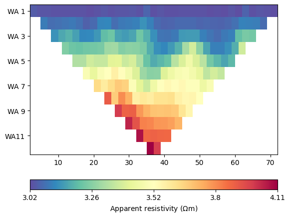
The data container has no apparent resistivities (token field ‘rhoa’) yet. We can let the Manager fix this later for us (as we now have the ‘k’ field), or we do it manually.

mgr.checkData(data)
print(data)

Data: Sensors: 38 data: 222, nonzero entries: ['a', 'b', 'k', 'm', 'n', 'r', 'rhoa', 'valid']

The data container does not necessarily contain data errors data errors (token field ‘err’), requiring us to enter data errors. We can let the manager guess some defaults for us automaticly or set them manually

data['err'] = ert.estimateError(data, relativeError=0.03, absoluteUError=5e-5)
# or manually:
# data['err'] = data_errors  # somehow
ert.show(data, data['err']*100)

(<Axes: >, <matplotlib.colorbar.Colorbar object at 0x7f2420852080>)

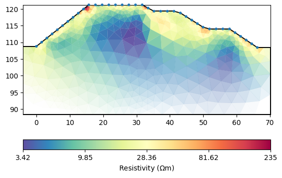
Now the data have all necessary fields (‘rhoa’, ‘err’ and ‘k’) so we can run the inversion. The inversion mesh will be created with some optional values for the parametric mesh generation.

mod = mgr.invert(data, lam=10, verbose=True,
                 paraDX=0.3, paraMaxCellSize=10, paraDepth=20, quality=33.6)

mgr.showResult()

fop: <pygimli.physics.ert.ertModelling.ERTModelling object at 0x7f2402c49120>
Data transformation: <pygimli.core._pygimli_.RTransLogLU object at 0x7f2402c489a0>
Model transformation: <pygimli.core._pygimli_.RTransLog object at 0x7f2402c487c0>
min/max (data): 6.07/33.48
min/max (error): 3.02%/4.11%
min/max (start model): 10.65/10.65
--------------------------------------------------------------------------------
inv.iter 0 ... chi² =  198.16
--------------------------------------------------------------------------------
inv.iter 1 ... chi² =   16.19 (dPhi = 90.28%) lam: 10.0
--------------------------------------------------------------------------------
inv.iter 2 ... chi² =    1.58 (dPhi = 80.44%) lam: 10.0
--------------------------------------------------------------------------------
inv.iter 3 ... chi² =    1.01 (dPhi = 11.83%) lam: 10.0
--------------------------------------------------------------------------------
inv.iter 4 ... chi² =    0.98 (dPhi = 0.53%) lam: 10.0


################################################################################
#                  Abort criterion reached: chi² <= 1 (0.98)                   #
################################################################################

(<Axes: xlabel='$x$ in m', ylabel='Depth in m'>, <matplotlib.colorbar.Colorbar object at 0x7f2423220a00>)

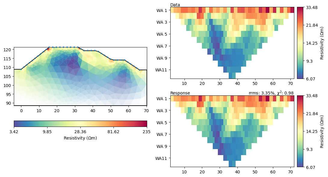
We can view the resulting model in the usual way.

mgr.showResultAndFit()
# np.testing.assert_approx_equal(ert.inv.chi2(), 1.10883, significant=3)

<Figure size 1100x600 with 6 Axes>

Or just plot the model only using your own options.

mgr.showResult(mod, cMin=5, cMax=30, cMap="Spectral_r", logScale=True)

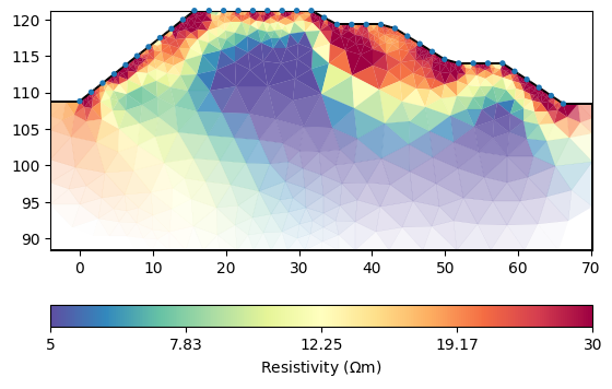
(<Axes: xlabel='$x$ in m', ylabel='Depth in m'>, <matplotlib.colorbar.Colorbar object at 0x7f2400e7bbe0>)