Structural coupled cooperative inversion (SCCI)

Joint inversion is an important method to improve resolution properties by combining different methods. Günther & Rücker (2006) and Günther et al. (2010) introduced a scheme later refined by Hellmann et al. (2017), Ronczka et al. (2017), and Skibbe et al. (2018, 2021).

We use the model already used in the pyGIMLi paper (Rücker et al., 2017) for petrophysical joint inversion.

We import the necessary libraries and the SCCI class

import os
import numpy as np
import pygimli as pg
from pygimli import meshtools as mt
from pygimli.physics import ert
from pygimli.physics import traveltime as tt
from pygimli.frameworks import SCCI
from pygimli.viewer.mpl.meshview import drawCWeight
from pygimli.physics.petro import transFwdArchieS as ArchieTrans
from pygimli.physics.petro import transFwdWyllieS as WyllieTrans

def createSynthModel(nSeg=32):
    """Return the modelling mesh, the porosity distribution and the
       parametric mesh for inversion.
    """
    # Create the synthetic model
    world = mt.createCircle(boundaryMarker=-1, nSegments=nSeg*2)
    tri = mt.createPolygon([[-0.8, -0], [-0.5, -0.7], [0.7, 0.5]],
                           isClosed=True, area=0.0015)
    c1 = mt.createCircle(radius=0.2, pos=[-0.2, 0.5], segments=16,
                         area=0.0025, marker=3)
    c2 = mt.createCircle(radius=0.2, pos=[0.32, -0.3], segments=16,
                         area=0.0025, marker=3)

    poly = mt.mergePLC([world, tri, c1, c2])

    poly.addRegionMarker([0.0, 0, 0], 1, area=0.0015)
    poly.addRegionMarker([-0.9, 0, 0], 2, area=0.0015)

    c = mt.createCircle(radius=0.99, nSegments=nSeg, start=np.pi, end=np.pi*3)
    [poly.createNode(p.pos(), -99) for p in c.nodes()]
    poly.save("poly.bms")
    mesh = pg.meshtools.createMesh(poly, q=34.4, smooth=[1, 10])
    mesh.scale(1.0/5.0)
    mesh.rotate([0., 0., 3.1415/3])
    mesh.rotate([0., 0., 3.1415])

    petro = pg.solver.parseArgToArray([[1, 0.9], [2, 0.6], [3, 0.3]],
                                      mesh.cellCount(), mesh)

    # Create the parametric mesh that only reflect the domain geometry
    world = mt.createCircle(boundaryMarker=-1, nSegments=nSeg*2, area=0.0051)
    paraMesh = pg.meshtools.createMesh(world, q=34.0, smooth=[1, 10])
    paraMesh.scale(1.0/5.0)

    return mesh, paraMesh, petro

mMesh, pMesh, saturation = createSynthModel()
rKW = dict(logScale=True, cMin=250, cMax=2500, cMap="Spectral_r")
vKW = dict(logScale=True, cMin=1000, cMax=2500, cMap="Spectral_r")
ertTrans = ArchieTrans(rFluid=20, phi=0.3)
res = ertTrans(saturation)
ttTrans = WyllieTrans(vm=4000, phi=0.3)
vel = 1./ttTrans(saturation)
sensors = mMesh.positions()[mMesh.findNodesIdxByMarker(-99)]

pg.info("Simulate ERT")
ERT = ert.ERTManager(verbose=False, sr=False)
ertScheme = ert.createERTData(sensors, schemeName='dd', closed=1)
ertData = ert.simulate(mMesh, scheme=ertScheme, res=res, noiseLevel=0.01)

pg.info("Simulate Traveltime")
TT = tt.TravelTimeManager(verbose=False)
ttScheme = tt.createRAData(sensors)
ttData = tt.simulate(mMesh, scheme=ttScheme, vel=vel, secNodes=5,
                     noiseLevel=0.001, noiseAbs=2e-6)

ERT = ert.ERTManager(ertData, verbose=True, sr=False)
ERT.setMesh(pMesh)

TT = tt.TravelTimeManager(ttData, verbose=True)
TT.errIsAbsolute = True
TT.setMesh(pMesh)

ERT.setRegularization(cType=1)

ERT.invert(zWeight=1, lam=100, maxIter=3)
# ERT.showResult(**rKW)

--------------------------------------------------------------------------------
--------------------------------------------------------------------------------
inv.iter 1 ... --------------------------------------------------------------------------------
inv.iter 2 ... --------------------------------------------------------------------------------
inv.iter 3 ...
976 [584.6820236994578,...,1826.2906069326712]

TT.invert(zWeight=1, lam=400, secNodes=5, startModel=1/2000, maxIter=3)
# ax, cb = TT.showResult(**vKW)
# ax.plot(pg.x(ttData), pg.y(ttData), "ko")

--------------------------------------------------------------------------------
--------------------------------------------------------------------------------
inv.iter 1 ... --------------------------------------------------------------------------------
inv.iter 2 ... --------------------------------------------------------------------------------
inv.iter 3 ...
976 [1567.0583593725025,...,1348.8951074640756]

scci = SCCI([ERT, TT], names=["ERT", "TT"])
scci.a = 0.1
scci.b = 0.02
scci.c = 1
scci.cmax = 100

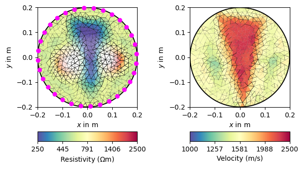
cw = scci.singleCWeights()
print(min(cw[0]), min(cw[1]), np.mean(cw[0]), np.mean(cw[1]))
fig, ax = pg.plt.subplots(ncols=2)
aa, cb = ERT.showResult(ax=ax[0], **rKW)
drawCWeight(aa, ERT.paraDomain, cw[0])
aa, cb = TT.showResult(ax=ax[1], **vKW)
drawCWeight(aa, TT.paraDomain, cw[1])
vPre = pg.Vector(TT.inv.model)
rPre = pg.Vector(ERT.inv.model)

0.22843373160888117 0.37792495225680195 0.6774758113067163 0.8326017170105604

TT.inv.lam = 1000
ERT.inv.lam = 200
scci.run(maxIter=5)  # save=True)
print(ERT.inv.chi2(), TT.inv.chi2())
print(min(ERT.inv.inv.cWeight()), min(TT.inv.inv.cWeight()))

Coupled inversion 1
Coupled inversion 2
Coupled inversion 3
Coupled inversion 4
Coupled inversion 5
1.2227427264621538 0.9653091652839475
0.37792495225680195 0.22843373160888117

ERT.inv.model = ERT.inv.inv.model()
TT.inv.model = 1./TT.inv.inv.model()
vPost = TT.inv.model
rPost = ERT.inv.model
print(rPre[0], rPost[0], pg.math.rrms(rPre, rPost))
print(vPre[0], vPost[0], pg.math.rms(vPre, vPost))

584.6820236994578 589.8011093042974 0.04705499190517188
1567.0583593725025 1572.4013312551738 65.94954888860734

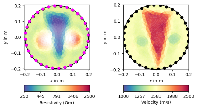
fig, ax = pg.plt.subplots(ncols=2)
aa, cb = ERT.showResult(ax=ax[0], **rKW)
aa.plot(pg.x(ttData), pg.y(ttData), "ko")
# drawCWeight(aa, ERT.paraDomain, ERT.inv.inv.cWeight())
aa, cb = TT.showResult(ax=ax[1], **vKW)
aa.plot(pg.x(ttData), pg.y(ttData), "ko")
# drawCWeight(aa, TT.paraDomain, TT.inv.inv.cWeight())

[<matplotlib.lines.Line2D object at 0x7f74c151f610>]

# References
#
# Günther, T., Dlugosch, R., Holland, R. & Yaramanci, U. (2010): Aquifer characterization using coupled inversion of DC/IP and MRS data on a hydrogeophysical test-site. - SAGEEP 23, 39 (2010); Keystone, CO.
# Günther, T. & Rücker, C. (2006): A new joint inversion approach applied to the combined tomography of dc resistivity and seismic refraction data. - Ext. abstract, 19. EEGS annual meeting (SAGEEP), 02.-06.04.2006; Seattle, USA.
# Hellman, K., Ronczka, M., Günther, T., Wennermark, M., Rücker, C. & Dahlin, T. (2017): Structurally coupled inversion of ERT and refraction seismic data combined with cluster-based model integration. Journal of Applied Geophysics 143, 169-181, doi:10.1016/j.jappgeo.2017.06.008.
# Ronczka, M., Hellman, K., Günther, T., Wisen, R., Dahlin, T. (2017): Electric resistivity and seismic refraction tomography, a challenging joint underwater survey at Aspö hard rock laboratory. Solid Earth 8, 671-682. doi:10.5194/se-8-671-2017.
# Rücker, C., Günther, T., Wagner, F.M. (2017): pyGIMLi: An open-source library for modelling and inversion in geophysics, Computers & Geosciences 109, 106-123, doi:10.1016/j.cageo.2017.07.011.
# Skibbe, N., Günther, T. & Müller-Petke, M. (2018): Structurally coupled cooperative inversion of magnetic resonance with resistivity soundings. Geophysics 83(6), JM51-JM63, doi:10.1190/geo2018- 0046.1.
# Skibbe, N., Günther, T. & Müller-Petke, M. (2021): Improved hydrogeophysical imaging by structural coupling of two-dimensional magnetic resonance and electrical resistivity tomography. Geophysics 86 (5), WB135-WB146, doi:10.1190/geo2020-0593.1.