3D Darcy flow

Here we illustrate Darcy flow in a heterogeneous 3D body. We use the general pygimli.solver.solveFiniteElements() to solve Darcy’s law:

\[\nabla \cdot(K \nabla p)=0\]

The sought hydraulic velocity distribution can then be calculated as the gradient field of \(\mathbf{v}=-\nabla p\).

import numpy as np
import pygimli as pg
import pygimli.meshtools as mt
from pygimli.viewer.pv import drawStreamLines, drawSlice

We start with creating the geometry: a small cube inside of a bigger one, and create a mesh from it.

plc = mt.createCube(size=[40, 20, 15], marker=1, boundaryMarker=0)
cube = mt.createCube(size=[15, 15, 8], marker=2, boundaryMarker=0)
geom = plc + cube

mesh = mt.createMesh(geom, area=4)

For the boundary conditions, we set the markers of all left boundaries to 1 and the markers of all righth boundaries to 2.

for bound in mesh.boundaries():
    x = bound.center().x()
    if x == mesh.xmin():
        bound.setMarker(1)
    elif x == mesh.xmax():
        bound.setMarker(2)

Next, we create a map for the hydraulic conductivity. The outer cube has 1e-4m/s and the inner 1e-6m/s.

kMap =[[1, 1e-4], [2, 1e-6]]
kArray = pg.solver.parseMapToCellArray(kMap, mesh)

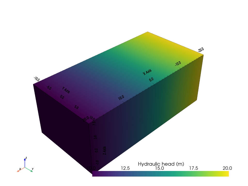
We set two different heads for the left and right bounday and solve the Darcy equation using Finite Elements

bc = {"Dirichlet": {1: 20.0, 2: 10.0}}
h = pg.solver.solveFiniteElements(mesh, kMap, bc=bc)

From the hydraulic head we compute the velocity by multiplying it with the hydraulic conductivity that is before transformed into an isotropic tensor.

kTensor = np.column_stack([kArray] * 3)
vel = -pg.solver.grad(mesh, h) * kTensor
pg.show(mesh, h, label="Hydraulic head (m)")

Static Scene

Interactive Scene

(<pyvista.plotting.plotter.Plotter object at 0x7fe1182ae650>, None)

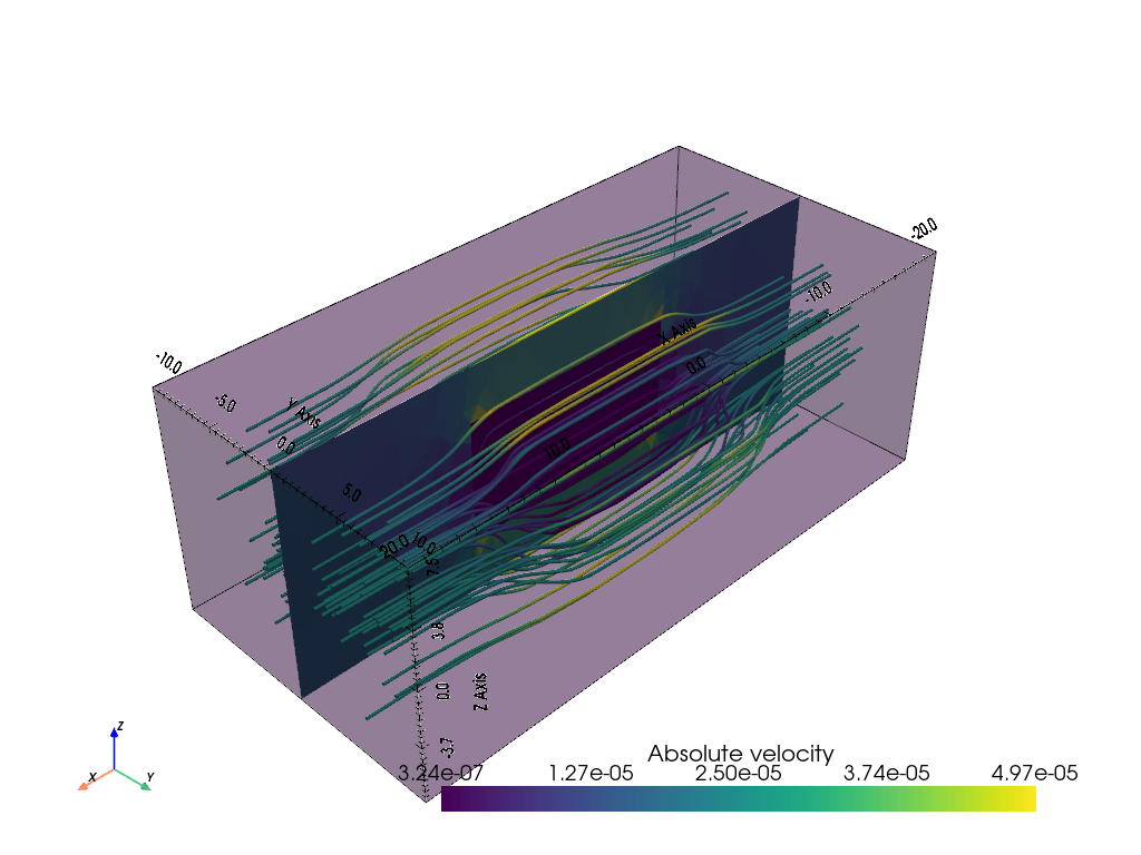
Last, we show the flow lines that avoid the poor conductor.

ax, _ = pg.show(mesh, alpha=0.3, hold=True, colorBar=False)
drawStreamLines(ax, mesh, vel, radius=.1, source_radius=10)
drawSlice(ax, mesh, normal=[0,1,0], data=pg.abs(vel), label="Absolute velocity")
ax.show()

Static Scene

Interactive Scene