Synthetic TDIP modelling and inversion

This example demonstrates the ERTIPManager introduced in pyGIMLi v1.4.3 for use with time-domain chargeability.

Whereas the classic ERTManager is for apparent resistivity only (that is inverted into a resistivity distribution), the ERTIPManager extends this by a simple IP component. This can be in the frequency domain (FD), i.e. apparent phase angle, or in the time domain, i.e. a chargeability.

Note that the ERT simulation can already simulate with complex (i.e. FD) resistivity, but not invert for it.

import numpy as np
import pygimli as pg
from pygimli.physics import ert
import pygimli.meshtools as mt

Synthetic model

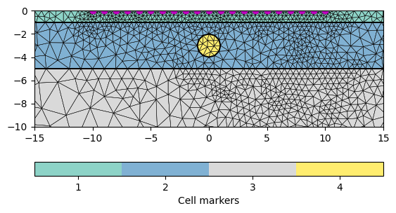
We build a layered model with layer boundaries at 1 and 5m depth. Additionally, we add a circle into the middle layer.

world = mt.createWorld(start=[-50, 0], end=[50, -50],
                       layers=[-1, -5], worldMarker=True)
scheme = ert.createData(elecs=pg.utils.grange(start=-10, end=10, n=21),
                        schemeName='dd')
circle = mt.createCircle(pos=[0, -3], radius=1, marker=4)
world += circle
for pos in scheme.sensorPositions():
    _= world.createNode(pos)
    _= world.createNode(pos + [0.0, -0.1])
mesh = mt.createMesh(world, quality=34.4)
ax, cb = pg.show(mesh, markers=True, showMesh=True, boundaryMarkers=False)
ax.plot(pg.x(scheme), pg.y(scheme), "mo")
ax.set_ylim(-10, 0)
ax.set_xlim(-15, 15)

(-15.0, 15.0)

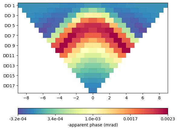
FD simulation

We associate different resistivities for the three layers and the identical resistivity for the circle, which is the only body with an imaginary component. First we create an FD data set for comparison using the normal simulate.

rhomap = [[1, 100. + 0j],
          [2, 50. + 0j],
          [3, 10.+ 0j],
          [4, 50.+ 1j]]

dataFD = ert.simulate(mesh, res=rhomap, scheme=scheme, verbose=True)
dataFD.show("phia", label="-apparent phase (mrad)")

(<Axes: >, <matplotlib.colorbar.Colorbar object at 0x7f40fa69c370>)

TD simulation

For time domain, we need a resistivity and a chargeability. Different from before, we specify them as vectors going from 0 to 4 (maximum cell marker). The simulate function first runs a DC forward calculation and then another (AC) computation. The results are stored in the rhoa and ma/ip data fields.

res = np.array([0, 100, 50, 10, 50.])
m = np.array([0, 0, 0, 0, 0.1])
mgr = ert.ERTIPManager()
dataTD = mgr.simulate(mesh=mesh, scheme=scheme, res=res, m=m)
dataTD.show("ip", label="-apparent chargeability")

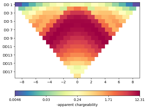
Mesh: Nodes: 1893 Cells: 3521 Boundaries: 5413 3521 3521

(<Axes: >, <matplotlib.colorbar.Colorbar object at 0x7f40f6173220>)

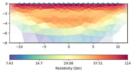
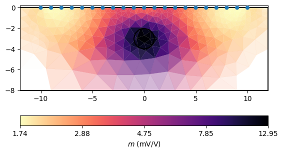
Inversion

We set a constant error and run an inversion with some keyword arguments. A TDIP inversion can be run by invertTDIP(). showResults show the resistivity result, whereas showIPModel shows the chargeability model. showResults shows both images below each other.

dataTD["err"] = 0.03
mgr = ert.ERTIPManager(dataTD)
mgr.invert(zWeight=0.2, quality=34.4, verbose=True)
mgr.showResult()
ax, cb = mgr.showIPModel()
pg.viewer.mpl.drawPLC(ax, circle, fitView=False, fillRegion=False)
# axs = mgr.showResults()

• 
• 

fop: <pygimli.physics.ert.ertModelling.ERTModelling object at 0x7f40f9e39530>
Data transformation: <pygimli.core._pygimli_.RTransLogLU object at 0x7f40f9e38b30>
Model transformation (cumulative):
         0 <pygimli.core._pygimli_.RTransLogLU object at 0x7f40f754c820>
min/max (data): 19.83/96.43
min/max (error): 3%/3%
min/max (start model): 54.62/54.62
--------------------------------------------------------------------------------
inv.iter 0 ... chi² =  171.39
--------------------------------------------------------------------------------
inv.iter 1 ... chi² =    2.38 (dPhi = 98.42%) lam: 20.0
--------------------------------------------------------------------------------
inv.iter 2 ... chi² =    0.67 (dPhi = 68.52%) lam: 20.0


################################################################################
#                  Abort criterion reached: chi² <= 1 (0.67)                   #
################################################################################
fop: <pygimli.physics.ert.ipModelling.DCIPMModelling object at 0x7f4130f62de0>
Data transformation: <pygimli.core._pygimli_.RTrans object at 0x7f40f754c8e0>
Model transformation: <pygimli.core._pygimli_.RTransLogLU object at 0x7f40f9e39cb0>
min/max (data): 4.6e-06/0.01
min/max (error): 11.12%/2.2e+04%
min/max (start model): 0.0021/0.0021
--------------------------------------------------------------------------------
inv.iter 0 ... chi² =   13.36
--------------------------------------------------------------------------------
inv.iter 1 ... chi² =    8.81 (dPhi = 28.08%) lam: 100.0
--------------------------------------------------------------------------------
inv.iter 2 ... chi² =    6.46 (dPhi = 8.92%) lam: 100.0
--------------------------------------------------------------------------------
inv.iter 3 ... chi² =    6.13 (dPhi = 1.36%) lam: 100.0
################################################################################
#                Abort criterion reached: dPhi = 1.36 (< 2.0%)                 #
################################################################################

(None, None)