3D modelling in a closed geometry#

This is a synthetic model of an experimental tank with a highly heterogeneous resistivity, motivated by the BAM Berlin.

Geometry: 0.99m x 0.5m x 1.0m Data: 48 Electrodes and 588 Measurements defined in modeltank.shm Each 24 electrodes are located at two opposite sides of the tank.

We use the pygimli meshtools to create a PLC of the tank and an inhomogeneity. The needed mesh is created by calling tetgen.

import numpy as np

import pygimli as pg
import pygimli.meshtools as mt
from pygimli.physics import ert

In contrast to field measurements, experimental tanks have well-defined spatial dimensions and need different boundary conditions (BC).

As there is no current flow through the tanks boundary at all, homogeneous (Neumann) BC are defined for the whole boundary. Neumann BC are natural (intrinsic) for the finite element simulations. link{tutorial:fem:bc}, so we just need to define a cube geometry including region markers.

plc = mt.createCube(size=[0.99, 0.5, 1.0], pos=[0.495, 0.25], boundaryMarker=1)

We first read the measuring scheme file and add the electrodes as nodes with the marker -99 to the geometry.

shm = pg.getExampleData("ert/modeltank.shm")

for s in shm.sensors():
    plc.createNode(s, marker=-99)

There are two small problems to overcome for simulating Neumann bodies.

First, we always need dipole current injection since there can be no current flow out of the closed boundaries of our experimental tank. (Note that by default single poles are simulated and superpositioned.) Therefore we define a reference electrode position inside the PLC, with a marker -999, somewhere away from the electrodes.

plc.createNode([0.5, 0.5, -0.5], marker=-999)

ID: 56, Marker: -999    RVector3: (0.5, 0.5, -0.5)

The second problem for pure Neumann domains is the non-uniqueness of the partial differential equation (there are only partial derivatives of the electric potential so an arbitrary value might be added, i.e. calibrated).

Therefore we add calibration node with marker -1000 where the potential is fixed , somewhere on the boundary and far from the electrodes.

plc.createNode([0.75, 0.25, 0.5], marker=-1000)

ID: 57, Marker: -1000   RVector3: (0.75, 0.25, 0.5)

For sufficient numerical accuracy it is generally a good idea to refine the mesh in the vicinity of the electrodes positions. We force the local mesh refinement by an additional node at 1 mm distance in -z-direction.

for s in plc.positions(pg.find(plc.nodeMarkers() == -99)):
    plc.createNode(s - [0.0, 0.0, 1e-3])

# Also refine the reference node
plc.createNode([0.5, 0.5, -0.5 - 1e-3])
#pg.show(plc, markers=True, showMesh=True)

ID: 106, Marker: 0      RVector3: (0.5, 0.5, -0.501)

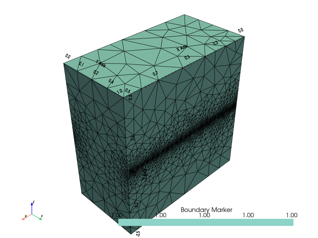
Create the tetrahedron mesh (calling the tetgen mesh generator)

mesh = mt.createMesh(plc)
pg.show(mesh, markers=True, showMesh=True)

Static Scene

Interactive Scene

(<pyvista.plotting.plotter.Plotter object at 0x7fe1161d4110>, None)

First we want to simulate our ERT response for a homogeneous resistivity of 1 :math:`Omega`m. Usually, simulate will calculate apparent resistivities (rhoa) and put them into the returned DataContainerERT. However, for the calculation of rhoa, geometric factors (k) are expected in the data container. If simulate does not find any k in the scheme file, it tries to determine them itself, either analytically (halfspace) or numerically (topography). Note that the automatic numerical calculating can only be a fallback mode. You usually want to keep full control about this calculation because you want the accuracy as high as possible by providing a special mesh with higher quality, lower max cell area, finer local mesh refinement, or quadratic base functions (p2).

We don’t want the automatic k generation here because we want also to demonstrate how you can solve this task yourself. The argument ‘calcOnly=True’ omits the check for valid k factors and will add the simulated voltages (u) in the returned DataContainerERT. The simulation current (i) is 1 A by default. In addition, the flag ‘sr=False’ omits the singularity removal technique (default) which not applicable in absence of (analytic) primary potential.

hom = ert.simulate(mesh, res=1.0, scheme=shm, sr=False,
                   calcOnly=True, verbose=True)

hom.save('homogeneous.ohm', 'a b m n u')

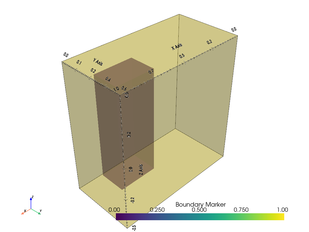
We now create an inhomogeneity (cube) and merge it with the above PLC. marker=2 ensures all cells of the cube being associated with a cell marker 2.

cube = mt.createCube(size=[0.3, 0.2, 0.8], pos=[0.7, 0.2], marker=2)
plc += cube

pg.show(plc, alpha=0.3)
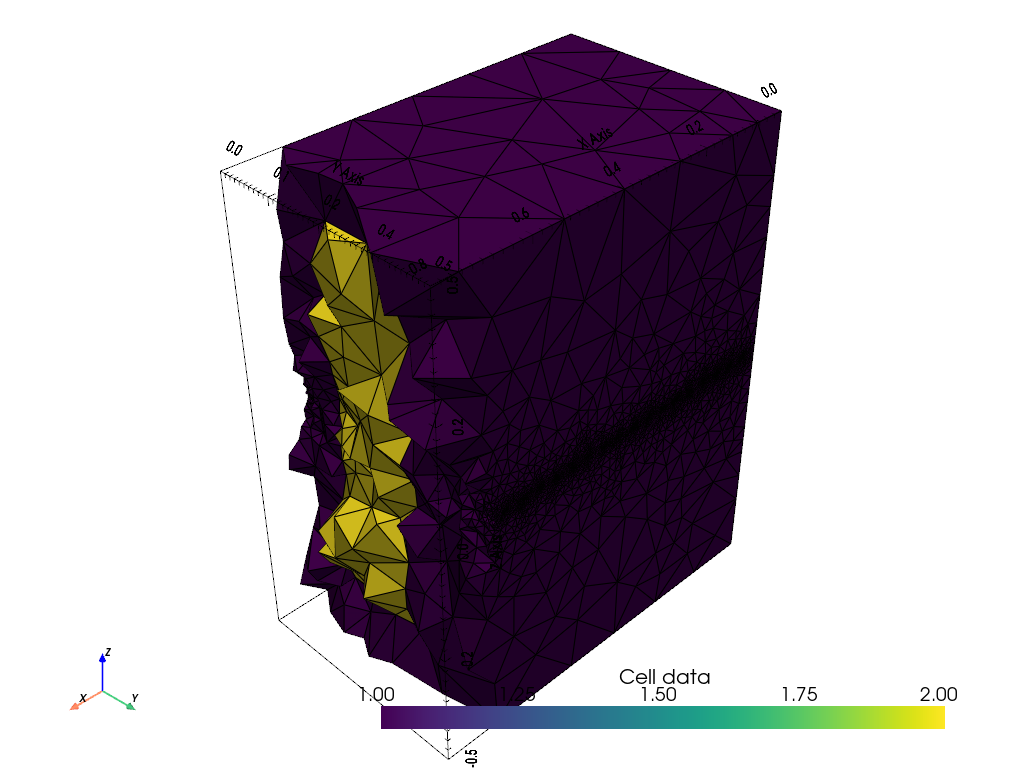
mesh = mt.createMesh(plc)

Static Scene

Interactive Scene

Also its advisable to control the geometry in a 3D viewer. We recommend Paraview https://www.paraview.org/ and will export the geometry and in the vtk file format.

# plc.exportVTK('plc')
# mesh.exportVTK('mesh')
pg.show(mesh, mesh.cellMarkers(), showMesh=True,
        filter={'clip':{'origin':(0.7, 0, 0.0)},})

Static Scene

Interactive Scene

(<pyvista.plotting.plotter.Plotter object at 0x7fe1161d9b50>, None)

Now that we have a mesh with different regions and cell markers, we can define a relationship between region marker and resistivity by defining a appropriate list. We also set sr=False here because singularity removal would need highly accurate primary potentials which can also only be calculated numerically.

res = [[1, 10.0], [2, 100.0]]  # map markers 1 and 2 to 10 and 100 Ohmm, resp.
het = ert.simulate(mesh, res=res, scheme=shm, sr=False,
                   calcOnly=True, verbose=True)

The apparent resistivity for a homogeneous model of 1 Ohmm should be 1 Ohmm. Therefore we can take the inverse of the modeled resistances for the homogeneous model and use it as geometric factors to find the apparent resistivities for the inhomogeneous model.

het['k'] = 1.0/ (hom('u') / hom('i'))
het['rhoa'] = het('k') * het('u') / het('i')

het.save('simulated.dat', 'a b m n rhoa k u i')

np.testing.assert_approx_equal(het['rhoa'][0], 9.5, 1)

# np.testing.assert_approx_equal(het('k')[0], 0.820615269548)

For such kind of simulations, the homogeneous part should be high accurate because it is usually needed once after storing the geometric factors. Note, do not forget to add some noise if you plan to invert such simulated data.