Note
Go to the end to download the full example code
Simple fit#
This tutorial shows how to do the simplest inversion case, a curve fit, by setting up a custom forward operator. The function to be fitted is`
with the two unknown coefficients A (a signal amplitude) and X (a decay rate). Both A and X are assumed to be positive which is often the case for physical properties. The easiest way to do this is via a logarithmic transformation of the model vector (containing A and X) which is very easily done in pyGIMLi.
First we import the pygimli library under a short name pg and the numerics library numpy. Additionally we load the python plotting module of the library matplotlib. Both are contained in most python distributions and systems.
import numpy as np
import matplotlib.pyplot as plt
import pygimli as pg
We set up the modelling operator, i.e. to return \({\bf f}({\bf x})\) for given model parameters A and X subsumed in a vector. In order to be able to use operator in inversion, we derive from the abstract modelling base class. The latter holds the main mimic of generating Jacobian and adminstrating the model, the regularization and so on. The only function to overwrite is response(). If no function createJacobian is provided, they are computed by brute force (forward calculations with altered parameters).
class ExpModelling(pg.Modelling):
    """Exponential decay function modelling operator."""
    def __init__(self, xvec, verbose=False):
        """Initialize with storing x values."""
        super().__init__()
        self.x = xvec

    def response(self, model):
        """Model response, i.e. A*exp(-x/x0)."""
        return model[0] * pg.exp(-self.x / model[1])

    def createStartModel(self, dataVals):
        return pg.Vector([1.0, 3.0])
The init function saves the x vector and defines the parameterization, i.e. two independent parameters (a 1D mesh with 1 cell and 2 properties). The response function computes the function using A=model[0] and X=model[1] The function startModel defines a meaningful starting vector. There are other methods to set the starting model as inv.setModel() but this one is a default one for people who use the class and forget about a starting model.
We first create an abscissa vector using numpy (note that pygimli also provides an exp function and generate synthetic data with two arbitrary A and X values.
We define an (absolute) error level and add Gaussian noise to the data.
error = 0.5
data += pg.randn(*data.shape) * error
Next, an instance of the forward operator is created. We could use it for calculating the synthetic data using f.response([10.5, 0.55]) or just f([10.5, 0.55]). We create a real-valued (R) inversion passing the forward operator, the data. A verbose boolean flag could be added to provide some output the inversion, another one prints more and saves files for debugging.
f = ExpModelling(x)
inv = pg.frameworks.MarquardtInversion(f)
We create a real-valued logarithmic transformation and apply it to the model. Similar could be done for the data which are by default treated linearly. We then set the error level that is used for data weighting. It can be a float number or a vector of data length. One can also set a relative error. Finally, we use an inversion style known as Marquardt scheme (pure local damping with decreasing the regularization parameter subsequently) and start with a relatively large regularization strength to avoid overshoot. Finally run yields the coefficient vector and we plot some statistics.
fop: <__main__.ExpModelling object at 0x7fe70891f1f0>
Data transformation: <pygimli.core._pygimli_.RTrans object at 0x7fe70a1b5cc0>
Model transformation: <pygimli.core._pygimli_.RTransLog object at 0x7fe70891fe70>
min/max (data): 1.24/10.42
min/max (error): 4.8%/40.25%
min/max (start model): 1/3
--------------------------------------------------------------------------------
inv.iter 0 ... chi² =   86.14
--------------------------------------------------------------------------------
inv.iter 1 ... chi² =   72.28 (dPhi = 16.08%) lam: 20.0
--------------------------------------------------------------------------------
inv.iter 2 ... chi² =   32.58 (dPhi = 54.93%) lam: 20.0
--------------------------------------------------------------------------------
inv.iter 3 ... chi² =    3.73 (dPhi = 88.56%) lam: 20.0
--------------------------------------------------------------------------------
inv.iter 4 ... chi² =    0.81 (dPhi = 78.30%) lam: 20.0
--------------------------------------------------------------------------------
inv.iter 5 ... chi² =    0.81 (dPhi = 0.19%) lam: 20.0
################################################################################
#                Abort criterion reached: dPhi = 0.19 (< 0.5%)                 #
################################################################################
16.24861653984905 0.8076697211961741
We see that after a few iterations the absolute rms value equals the noise level corresponding to a chi-squared misfit value of 1 as it should be the case for synthetic data. The relative rms (in %) is less relevant here but can be for other applications. Additionally the ranges for model and model response are given and the objective function consisting of data misfit and model roughness times lambda. Note that due to the local regularization the second term does not contribute to Phi.
We finally create a plotting figure and plot both data and model response.
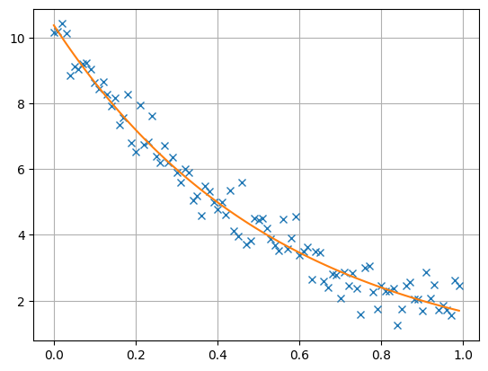
The resulting model vector has a length of 2 and consists of the inverted A and X values that are close to the synthetic values, being equivalent within error bounds.
print(coeff)
2 [10.372498358712114, 0.5467344595857115]
If you are interested which way the inversion took, you can have a look at the model history.
for model in inv.modelHistory:
    print(model)

plt.show()
2 [1.0, 3.0]
2 [1.5446513082933024, 2.4761221423780158]
2 [4.139259790264265, 0.9302882509465832]
2 [9.745161686229341, 0.45065983072159094]
2 [10.31785519142258, 0.5502649587666306]
2 [10.372498358712114, 0.5467344595857115]