1.2. First steps

The modelling as well as the inversion part of pyGIMLi often requires a spatial discretization for the domain of interest, the so called GIMLI::Mesh. This tutorial shows some basic aspects of handling a mesh.

First, the library needs to be imported. To avoid name clashes with other libraries we suggest to import pygimli and alias it to the simple abbreviation pg: CR

import pygimli as pg

Every part of the c++ namespace GIMLI is bound to python and can be used with the leading pg.

For instance get the current version for pyGIMLi with:

print(pg.__version__)

1.5.5.post2+6.gad7b1cc9

Now that we know the name space GIMLI, we can create a first mesh. A mesh is represented by a collection of nodes, cells and boundaries, i.e., geometrical entities.

Note

A regularly spaced mesh consisting of rectangles or hexahedrons is usually called a grid. However, a grid is just a special variant of a mesh so GIMLi treats it the same. The only difference is how they are created.

GIMLi provides a collection of tools for mesh import, export and generation. A simple grid generation is built-in but we also provide wrappers for unstructured mesh generations, e.g., Triangle, Tetgen and Gmsh. To create a 2d grid you need to give two arrays/lists of sample points in x and y direction, in that order, or just numbers.

grid = pg.createGrid(x=[-1.0, 0.0, 1.0, 4.0], y=[-1.0, 0.0, 1.0, 4.0])

The returned object grid is an instance of GIMLI::Mesh and provides various methods for modification and io-operations. General information about the grid can be printed using the simple print() function.

print(grid)

Mesh: Nodes: 16 Cells: 9 Boundaries: 24

Or you can access them manually using different methods:

print('Mesh: Nodes:', grid.nodeCount(),
      'Cells:', grid.cellCount(),
      'Boundaries:', grid.boundaryCount())

Mesh: Nodes: 16 Cells: 9 Boundaries: 24

You can iterate through all cells of the general type GIMLI::Cell that also provides a lot of methods. Here we list the number of nodes and the node ids per cell:

for cell in grid.cells():
    print("Cell", cell.id(), "has", cell.nodeCount(),
          "nodes. Node IDs:", [n.id() for n in cell.nodes()],
          "Position:", cell.center())

print(type(grid.cell(0)))

Cell 0 has 4 nodes. Node IDs: [0, 1, 5, 4] Position: RVector3: (-0.5, -0.5, 0.0)
Cell 1 has 4 nodes. Node IDs: [1, 2, 6, 5] Position: RVector3: (0.5, -0.5, 0.0)
Cell 2 has 4 nodes. Node IDs: [2, 3, 7, 6] Position: RVector3: (2.5, -0.5, 0.0)
Cell 3 has 4 nodes. Node IDs: [4, 5, 9, 8] Position: RVector3: (-0.5, 0.5, 0.0)
Cell 4 has 4 nodes. Node IDs: [5, 6, 10, 9] Position: RVector3: (0.5, 0.5, 0.0)
Cell 5 has 4 nodes. Node IDs: [6, 7, 11, 10] Position: RVector3: (2.5, 0.5, 0.0)
Cell 6 has 4 nodes. Node IDs: [8, 9, 13, 12] Position: RVector3: (-0.5, 2.5, 0.0)
Cell 7 has 4 nodes. Node IDs: [9, 10, 14, 13] Position: RVector3: (0.5, 2.5, 0.0)
Cell 8 has 4 nodes. Node IDs: [10, 11, 15, 14] Position: RVector3: (2.5, 2.5, 0.0)
<class 'pygimli.core.libs._pygimli_.Quadrangle'>

Similarly, you can iterate through all

for node in grid.nodes()[:3]:
    print("Node", node.id(), "at", node.pos())

Node 0 at RVector3: (-1.0, -1.0, 0.0)
Node 1 at RVector3: (0.0, -1.0, 0.0)
Node 2 at RVector3: (1.0, -1.0, 0.0)

or boundaries

for bnd in grid.boundaries()[:3]:
    print("Boundary", bnd.id(),
          "at center", bnd.center(),
          "directing at", bnd.norm())

print(type(grid.boundary(0)))

Boundary 0 at center RVector3: (-0.5, -1.0, 0.0) directing at RVector3: (-0.0, -1.0, 0.0)
Boundary 1 at center RVector3: (0.0, -0.5, 0.0) directing at RVector3: (1.0, 0.0, 0.0)
Boundary 2 at center RVector3: (-0.5, 0.0, 0.0) directing at RVector3: (-0.0, 1.0, 0.0)
<class 'pygimli.core.libs._pygimli_.Edge'>

Note that the node numbers can be more easily accessed by pg.x(grid) etc.

To generate the input arrays x and y, you can use the built-in GIMLI::Vector (pre-defined with values that are type double as pg.Vector), standard python lists or numpy arrays, which are widely compatible with pyGIMLi vectors.

import numpy as np

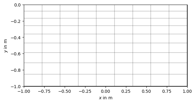
grid = pg.createGrid(x=np.linspace(-1.0, 1.0, 10),
                     y=1.0 - np.logspace(np.log10(1.0), np.log10(2.0), 10))

This new grid contains

print(grid.cellCount())

81

rectangles of type GIMLI::Quadrangle derived from the base type GIMLI::Cell, edges of type GIMLI::Edge, which are boundaries of the general type GIMLI::Boundary, counting to

print(grid.boundaryCount())

180

The mesh can be saved and loaded in our binary mesh format .bms. Or exported into .vtk format for 2D or 3D visualization using Paraview.

However, we recommend visualizing 2-dimensional content using Python scripts that provide better exports to graphics files (e.g., png, pdf, svg). pygimli provides basic post-processing routines using the matplotlib visualization package. The main visualization call is pygimli.viewer.show, or shortly pg.show() which is sufficient for most meshes, fields, models and streamline views.

pg.show(grid)

(<Axes: xlabel='$x$ in m', ylabel='$y$ in m'>, None)

pg.wait()