6. Modelling

As the Finite Element analysis (FEA) is the most commonly used numerical method used, this tutorial covers this method, referring the M (Modelling) in pyGIMLi.

6.1. Finite Elements for Poisson equation

Details on the theory of the Finite Elements Analysis (FEA) can be found in several books, e.g., [Zienkiewicz, 1977]. Nevertheless, we provide a brief overview of the main concepts and ideas behind FEA to solve boundary value problems.

Assume Poisson’s equation as the simplest partial differential equation (PDE) to be solved for the scalar field \( u(\mathbf{r}) \) within a modelling domain \({r}\in\Omega\) with a source \(f\).

\[ - \nabla \cdot a \nabla u = f \quad{\mathrm{in}}~\Omega \]

The generalized Poisson operator \(\Delta = \nabla\cdot\nabla\), i.e., the divergence of the flow (gradient times some conductivity), is a second-order partial derivative of the field \(u(\mathbf{r})\) in Cartesian coordinates, i.e., in 1D \( \mathbf{r} = (x) \), in 2D \( {r} = (x, y) \), or in 3D space \( \mathbf{r} = (x, y, z) \). On the boundary \(\partial\Omega\) of the domain, we assume known values of \(u=u_B\) (Dirichlet boundary conditions) or gradients \(\partial u/\partial n=g_B\).

A common approach to solve this problem is the method of weighted residuals. An approximated solution \( u_h\approx u\) satisfies the PDE with a remainder \(R=\Delta u_h + f\). We choose some weighting functions \(w\) and minimize \(R\) over our modelling domain:

\[ \int_{\Omega} w R = 0\; \]

which leads to

\[ \int_{\Omega} - w \nabla \cdot a \nabla u_h = \int_{\Omega} w f \]

It is preferable to eliminate the second derivative in the Laplace operator, either through to integration by parts or by applying the product rule and Gauss’s law. This leads to the so-called weak formulation:

\[ \int_{\Omega} a \nabla u_h \cdot \nabla w - \int_{\partial \Omega} a w \mathbf{n} \cdot \nabla u_h = \int_{\Omega} w f \]

\[ \int_{\Omega} a \nabla u_h \cdot \nabla w = \int_{\Omega} w f + \int_{\partial \Omega} a w \frac{\partial u_h}{\partial\mathbf{n}} \]

We choose a function basis to approximate \(u_h\):

\[ u_h = \sum_i^\mathcal{N} \mathrm{u}_i N_i \]

This fundamental relation discretizes the continuous solution \(u_h\) by a vector of discrete coefficients \(\mathrm{u} = \{\mathrm{u}_i\} \) for a number \(\mathcal{N}\) degrees of freedom (dof). The basis functions \(N_i\) can be understood as interpolation rules describing the solution on the whole domain, spanned by nodes, edges or faces in a mesh. Mostly, \(N_i\) represent nodal basis functions (e.g. hat functions) so that the \(\mathrm{u}_i\) correspond to the solution at nodes.

Now we can set the unknown weighting functions to be identical to the basis functions \(w=N_j\) (Galerkin method) so that \( \forall j=0\ldots\mathcal{N} \) holds

\[ \int_{\Omega} a \sum_i \nabla N_i \cdot \nabla N_j \mathrm{u}_i = \int_{\Omega} f_j N_j + \int_{\partial \Omega} g N_j \quad \text{with}\quad g = \frac{\partial u}{\partial \mathbf{n}} \]

For \(g=0\) (natural Neumann boundary conditions) this can be rewritten as

\[ \mathrm{A} \mathrm{u} = \mathrm{b} \]

with \(\mathrm{A}\) referred to as Stiffness matrix

\[ \mathrm{A} = \{\mathrm{a}_{i,j}\} = \int_{\Omega}\nabla N_i \cdot \nabla N_j \]

and the right hand \(\mathrm{b}\) side known as load vector

\[ \mathrm{b} = \{\mathrm{b}_j\} = \int_{\Omega} f_j N_j \]

The solution of this linear system of equations leads to the discrete solution \( \mathrm{u} = \{\mathrm{u}_i\} \) for all \( i=1\ldots\mathcal{N}\) dofs spanning the modelling domain.

The choice of the dofs is crucial. If we choose too few, the accuracy of the sought solution might be pool. If we choose too many, the dimension of the system matrix will become large, leading to higher memory consumption and computation times.

To define the nodes, we discretize our modelling domain into cells, or the eponymous elements. Cells are basic geometric shapes like triangles or hexahedrons and are constructed from the nodes and collected in a mesh. For more details, refer to the Meshes section.

To complete the solution for the small example, we still need to apply the boundary condition \(u=u_B\) which is known as the Dirichlet condition. Setting explicit values for our solution is not covered by the general Galerkin weighted residuum method but we can solve it algebraically. We reduce the linear system of equations by the known solutions \(u_B={u_k}\) for all \(k\) nodes on the affected boundary elements:

\[\begin{split} \mathrm{A_D}\cdot\mathrm{u} = \mathrm{b_D} \\ \text{with } \mathrm{A_D} = \{\mathrm{a}_{i,j}\}\quad\forall i, j ~\notin~ k ~\text{and}~1~\forall~i,j \in k\\ \mathrm{b_D} = \{\mathrm{b}_j\} - \mathrm{A}\cdot\mathrm{g}\quad\forall j \notin k~\text{and}~u_k~\forall~j \in k \end{split}\]

Now we have all parts for assembling \(\mathrm{A_D}\) and \(\mathrm{b_D}\) and finally solve the given boundary value problem for the interior points.

It is usually a good idea to test a numerical approach with known solutions. To keep things simple, we create a modelling problem from the reverse direction (method of manufactured solution). We choose a solution, calculate the right hand side function and select the domain geometry suitable for nice Dirichlet values.

\[ u(x,y) = \operatorname{sin}(x)\operatorname{sin}(y) \]

\[ - \Delta u = f(x,y) = 2 \operatorname{sin}(x)\operatorname{sin}(y) \]

\[ \Omega \in I\!R^2 \quad \text{on}\quad 0 \leq x \leq 2\pi,~~ 0 \leq y \leq 2\pi \]

\[ u = g = 0 \quad \text{on}\quad \partial \Omega \]

We now can solve the Poison equation applying the FEA capabilities of pygimli and compare the resulting approximate solution \(\mathrm{u}\) with our known exact solution \(u(x,y)\).

6.2. Boundary conditions (BC)

After importing the necessary modules

Show code cell content

Hide code cell content

import numpy as np
import pygimli as pg

from pygimli.solver import solve
from pygimli.viewer import show
from pygimli.viewer.mpl import drawStreams
import pygimli.meshtools as mt

we create a grid to do some modelling on.

grid = pg.createGrid(x=np.linspace(-1.0, 1.0, 21),
                     y=np.linspace(-1.0, 1.0, 21))
grid.show(boundaryMarkers=True)
print(grid)

Mesh: Nodes: 441 Cells: 400 Boundaries: 840

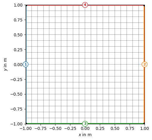
By default, all cells have the same marker, but the boundary markers are numbered from 1 to 4 for attributing .

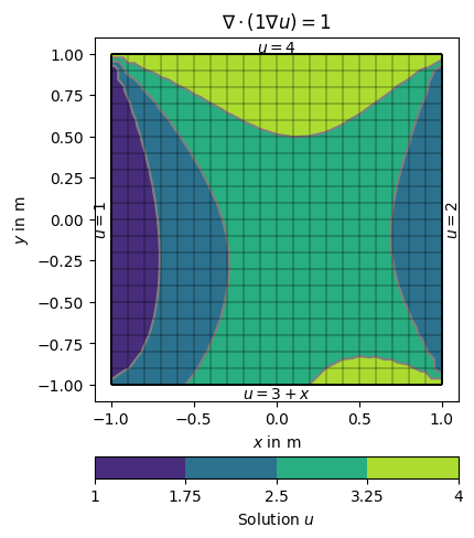
There are different ways of specifying BCs. They can be maps from markers to values, explicit functions or implicit (lambda) functions. We use the example of the Poisson equation on the unit square and specify different boundary conditions on the four sides.

• The boundaries 1 (left) and 2 (right) are directly mapped to the values 1 and 2.

• On side 3 (top), a lambda function 3+x is used (p is the boundary position and p[0] its \(x\) coordinate).

• On side 4 (bottom), a function uDirichlet is used that simply returns 4 in this example but can compute anything as a function of the individual boundary b.

def uDirichlet(boundary):
    """Return a solution value for a given boundary.
        Scalar values are applied to all nodes of the boundary."""
    return 4.0

dirichletBC = {1: 1,                                           # left
               2: 2.0,                                         # right
               3: lambda boundary: 3.0 + boundary.center()[0], # bottom
               4: uDirichlet}                                  # top

The boundary conditions are passed using the BC keyword dictionary dirichletBC.

u = solve(grid, f=1., bc={'Dirichlet': dirichletBC})

# Note that showMesh returns the figure axes and the colorBar.
ax, cbar = show(grid, data=u, label='Solution $u$')

show(grid, ax=ax)

ax.text(1.02, 0, '$u=2$', va='center', ha='left',  rotation='vertical')
ax.text(-1.01, 0, '$u=1$', va='center', ha='right', rotation='vertical')
ax.text(0, 1.01, '$u=4$', ha='center')
ax.text(0, -1.01, '$u=3+x$', ha='center', va='top')

ax.set_title('$\\nabla\cdot(1\\nabla u)=1$')

ax.set_xlim([-1.1, 1.1])  # some boundary for the text
ax.set_ylim([-1.1, 1.1]);

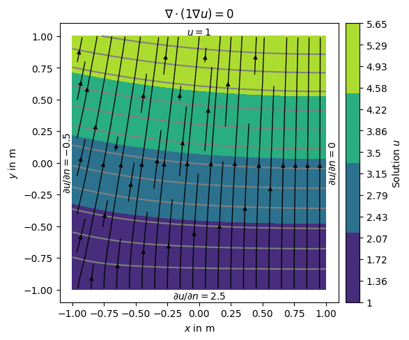
Alternatively, we can define the gradients of the solution on the boundary, i.e., Neumann type BC. This is done through another dictionary {marker: value} passed along Dirichlet with the bc keyword.

neumannBC = {1: -0.5,  # left
             4: 2.5}  # bottom

dirichletBC = {3: 1.0}  # top

u = solve(grid, f=0., bc={'Dirichlet': dirichletBC, 'Neumann': neumannBC})

Note that on boundary 2 (right) has no BC explicitly applied leading to default (natural) BC that are of homogeneous Neumann type \(\frac{\partial u}{\partial n}=0\)

ax = show(grid, data=u, filled=True, orientation='vertical',
          label='Solution $u$',
          levels=np.linspace(min(u), max(u), 14), hold=True)[0]

# add streamlines to show the gradients of (i.e., the flow direction).
drawStreams(ax, grid, u)
ax.text(0.0, 1.01, '$u=1$',
        horizontalalignment='center')  # top -- 3
ax.text(-1.0, 0.0, '$\partial u/\partial n=-0.5$',
        va='center', ha='right', rotation='vertical')  # left -- 1
ax.text(0.0, -1.01, '$\partial u/\partial n=2.5$',
        ha='center', va='top')  # bot -- 4
ax.text(1.01, 0.0, '$\partial u/\partial n=0$',
        va='center', ha='left', rotation='vertical')  # right -- 2

ax.set_title('$\\nabla\cdot(1\\nabla u)=0$')

ax.set_xlim([-1.1, 1.1])
ax.set_ylim([-1.1, 1.1]);

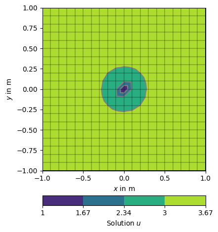
Its also possible to force single nodes to fixed values.

node0 = grid.findNearestNode([0.0, 0.0])
u = solve(grid, f=1., bc={'Node': [node0, 1.0]})
np.testing.assert_approx_equal(u[node0], 1.0, significant=10)

ax, _ = pg.show(grid, u, logScale=False, label='Solution $u$',)
_ = pg.show(grid, ax=ax)

6.3. Modelling in the halfspace

In most cases, we want to model the subsurface below the Earth’s surface. To this end, we use functions from the pygimli.meshtools module to create a PLC (e.g. including topography) and generate a mesh from it. There are so-called world boundaries that define the surface and bottom of the modelling domain with predefined values.

world = mt.createWorld(start=[-50, 0], end=[50, -30],
                       layers=[-10, -30], worldMarker=True)
_ = world.show(markers=True, boundaryMarkers=True)

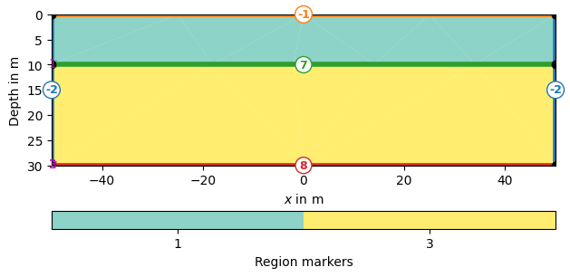
Definition of Boundary Conditions

• Boundary marker (-1) : surface boundary conditions - pg.core.MARKER_BOUND_HOMOGEN_NEUMANN

• Boundary marker (-2) : mixed-boundary conditions - pg.core.MARKER_BOUND_MIXED

• Boundary marker ( >= 1 ) : no-flow boundaries