7. Visualization#
As presented in the Fundamentals, pyGIMLi offers some basic post-processing routines for plotting. For 2D and 3D visualizations, we rely on Matplotlib and pyVista, respectively, and provide the following frameworks:
Drawing functions using Matplotlib. |
|
Pyvista based drawing functions used by pygimli.viewer. |
In the following, we will give a brief overview on the most important aspects on visualizing your plots as well as performing simple (cosmetic) changes.
7.1. Plotting in 2D#
For plotting in 2D, the method pygimli.viewer.showMesh() is called, which creates an axis object and plots a 2D mesh, if provided with node or cell data. As already discussed in the fundamentals section, the type of data determines the appropriate draw method.
This matplotlib glossary comprehends all possible adjustments that you can apply to plots based on pg.show(). In the following table, we summarized the most relevant functions:
|
|
|
|
|
|
|
|
|
|
|
|
|
|
|
|
|
|
|
|
|
|
|
|
|
|
|
|
|
|
|
|
|
|
|
|
|
7.1.1. Plotting meshes and models#
As described in the Fundamentals section, pygimli.viewer.show() and pygimli.viewer.showMesh() utilize a variety of drawing functions, depending on the input data provided. In the following, we will take a look at how to manually access the necessary drawing functions to plot an empty mesh, as well as cell-based and node-based data.
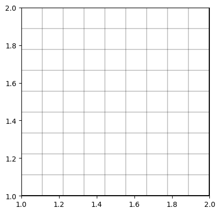
To visualize a grid or a triangular mesh in 2D, we can simply make use of the pygimli.viewer.show() function, which refers to pygimli.viewer.mpl.drawMesh():
n = np.linspace(1, 2, 10)
mesh = pg.createGrid(x=n, y=n)
fig, ax = plt.subplots()
mpl.drawMesh(ax, mesh)
plt.show()
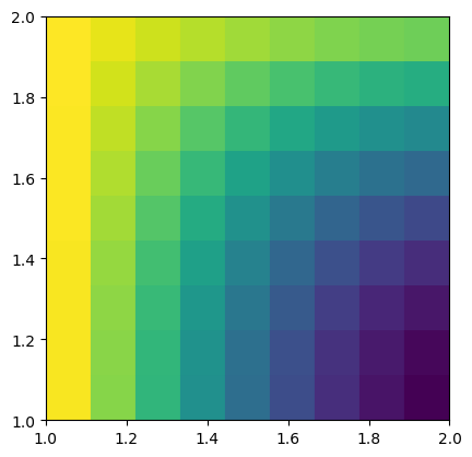
If we now want to plot cell-based values on top of our mesh, pygimli.viewer.show() links to the function pygimli.viewer.mpl.drawModel():
mx = pg.x(mesh.cellCenter())
my = pg.y(mesh.cellCenter())
data = np.cos(1.5 * mx) * np.sin(1.5 * my)
fig, ax = plt.subplots()
mpl.drawModel(ax, mesh, data)
plt.show()
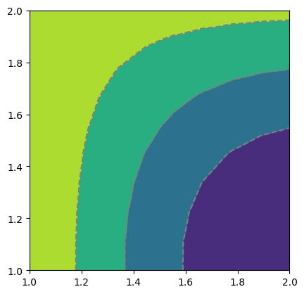
Simliarly, for scalar field values, the function pygimli.viewer.mpl.drawField() is utilized:
nx = pg.x(mesh.positions())
ny = pg.y(mesh.positions())
data = np.cos(1.5 * nx) * np.sin(1.5 * ny)
fig, ax = plt.subplots()
mpl.drawField(ax, mesh, data)
plt.show()
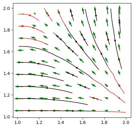
pyGIMLi also allows to plot vector field streamlines with pygimli.viewer.mpl.drawStreams, as in the following example. Every cell contains only one streamline and every new stream line starts in the center of a cell.
fig, ax = plt.subplots()
mpl.drawStreams(ax, mesh, data, color='red')
mpl.drawStreams(ax, mesh, data, dropTol=0.9)
mpl.drawStreams(ax, mesh, pg.solver.grad(mesh, data),
color='green', quiver=True)
ax.set_aspect('equal')
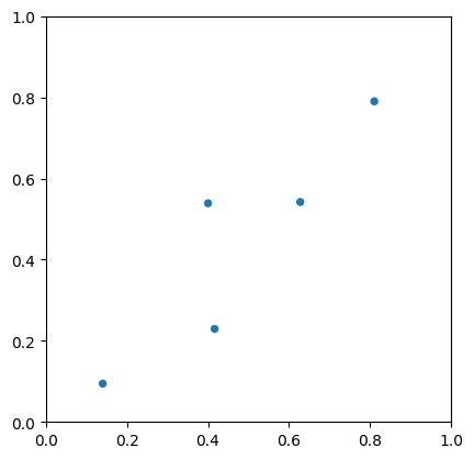
A more specific case is the visualization of sensor positions, which is also covered by a drawing function within the visualization framework of pyGIMLi. By providing a list of sensor positions to plot as [x,y] pairs, the function pygimli.viewer.mpl.drawSensors()draws the sensor positions as dots with a given diameter.
sensors = np.random.rand(5, 2)
fig, ax = pg.plt.subplots()
mpl.drawSensors(ax, sensors, diam=0.02, coords=[0, 1])
ax.set_aspect('equal')
7.2. Plotting in 3D#
For plotting in 3D, pyGIMLi utilizes the pygimli.viewer.pv module, which leverages the capabilities of pyVista for rendering. The primary function for visualizing 3D meshes is pygimli.viewer.pv.drawMesh(), which can handle various types of 3D data, including cell-based and node-based data. Similar to 2D plotting, the type of data provided determines the appropriate drawing method. As for the 2D plots, we can fine-tune the 3D plots by referring to the pyvista.Plotter functions
The following examples demonstrate how to plot 3D meshes, cell data, and streamlines, as well as how to create slices through the mesh for detailed analysis.
7.2.1. Plotting meshes and models in 3D#
Plotting meshes using pyVista is straightforward with pyGIMLi. The pygimli.viewer.pv.drawMesh() function is called to visualize 3D meshes and models, leveraging pyVista’s powerful rendering capabilities.
from pygimli.viewer import pv
plc = mt.createCube(size=[40, 20, 15], marker=1, boundaryMarker=0)
cube = mt.createCube(size=[15, 15, 8], marker=2, boundaryMarker=0)
geom = plc + cube
mesh = mt.createMesh(geom, area=4)
pg.show(mesh, style='wireframe', showMesh=True)
Opening /tmp/tmps_0fi_9o.poly.
Segments are connected properly.
(<pyvista.plotting.plotter.Plotter at 0x1533ad3f8cd0>, None)
To visualize cell-based values in a 3D mesh created with pyVista, pg.show makes use of the pygimli.viewer.pv.drawModel() function, which draws a given mesh together with provided values:
mx = pg.x(mesh.cellCenter())
my = pg.y(mesh.cellCenter())
mz = pg.z(mesh.cellCenter())
data = mx
pg.show(mesh, data, label="Cell position x (m)")
(<pyvista.plotting.plotter.Plotter at 0x15339dd69f10>, None)
As for the 2D section, pyVista also allows to plot streams by taking vector field of gradient data per cell. The according function is utilized in the example below:
ax, _ = pg.show(mesh, alpha=0.3, hold=True, colorBar=False)
pv.drawStreamLines(ax, mesh, data, radius=.1, source_radius=10)
ax.show()
Creating slices in a 3D plot allows for detailed analysis of the internal structure of the mesh. The pygimli.viewer.pv.drawSlice() function can be used to create and visualize these slices, specifying the normal vector and cell values to be displayed.
ax, _ = pg.show(mesh, alpha=0.3, hold=True, colorBar=False)
pv.drawSlice(ax, mesh, normal=[0,1,0], data=data, label="Cell position x")
ax.show()
If you want to take a look at more practical applications and examples that fully use the plotting capabilities of pyGIMLi, please refer to the examples section.
7.3. External plotting#
If you ever encounter the situation that the plotting capabilities of pyGIMLi are too limited for your need and you want to use more powerful programs such as Paraview, you can easily export meshes and models from pyGIMLi.
The VTK format can save values along with the mesh, point data like voltage under POINT_DATA and cell data like velocity under CELL_DATA. It is particularly suited to save inversion results including the inversion domain in one file.