3. Data#
3.1. The DataContainer class#
Data are often organized in a data container storing the data values in named vectors as well as the geometry of source and receivers. Like a dictionary, the names of the contained arrays are arbitrary and depend on the available information and method. Additionally to the data vectors, it stores sensor geometry and can story additional geometric data like topography.
Similar to a pandas dataframe, all vectors are guaranteed to be of the same size determined by the size() method, and can be filtered. By default, they are (float) vectors but can also be indices into the sensor geometry to indicate the sensor number. Let’s first create a DataContainer from scratch, assume we want to create and store Vertical Electrical Sounding (VES) data.
We define logarithmically equidistant AB/2 spacings.
ab2 = np.logspace(0, 3, 11)
print(ab2)
[   1.            1.99526231    3.98107171    7.94328235   15.84893192
   31.6227766    63.09573445  125.89254118  251.18864315  501.18723363
 1000.        ]
We create an empty data container and feed some data into it just like in a dictionary or dataframe.
ves_data = pg.DataContainer()
ves_data["ab2"] = ab2
ves_data["mn2"] = ab2 / 3
print(ves_data)
Data: Sensors: 0 data: 11, nonzero entries: ['ab2', 'mn2']
One can also use .showInfos() to see the content of the data container with more wording.
ves_data.showInfos()
Sensors: 0, Data: 11
SensorIdx:  Data: ab2 mn2 valid
As you can see, out there is no sensor information. In the next subsection we will explain how to add sensor information to a data container.
Note
DataContainers can also be defined for specific methods with predefined names for sensors and necessary data names. For example pygimli.physics.ert.DataContainer already has 'a', 'b', 'm', 'n' index entries. One can also add alias translators like 'C1', 'C2', 'P1', 'P2', so that dataERT[‘P1’] will return dataERT[‘m’] etc.
3.2. Creating Sensors#
Assume we have data associated with a transmitter, some receivers and some properties. The transmitter (Tx) and receiver (Rx) positions are stored separately and we refer them with an Index (integer). Therefore we define these fields as index fields.
data = pg.DataContainer()
data.registerSensorIndex("Tx")
data.registerSensorIndex("Rx")
Then we create a list of ten sensors with a 2m spacing. We can create sensors at any moment as long as it is not in the same position of an existing sensor.
for x in np.arange(10):
    data.createSensor([x*2, 0])

print(data)
Data: Sensors: 10 data: 0, nonzero entries: ['Rx', 'Tx']
We want to use all of them (and two more!) as receivers and a constant transmitter of number 2.
data["Rx"] = np.arange(12) # defines size
# data["Tx"] = np.arange(9) # does not work as size matters!
data["Tx"] = pg.Vector(data.size(), 2)
print(data)
Data: Sensors: 10 data: 12, nonzero entries: ['Rx', 'Tx']
Obviously there are two invalid receiver indices (10 and 11) as we only created sensors up to index 9. We can check the validity of the data container and remove invalid entries.
data["valid"] = 1  # set all values
data.checkDataValidity()
data.removeInvalid()
print(data)
Data: Sensors: 10 data: 10, nonzero entries: ['Rx', 'Tx', 'valid']
Warning: removed 2 values due to sensor index out of bounds!
Data validity check: found 2 invalid data.
Data validity check: remove invalid data.
We can filter the data by logical operations
data.remove(data["Rx"] == data["Tx"])
print(data)
Data: Sensors: 10 data: 9, nonzero entries: ['Rx', 'Tx', 'valid']
To store some data like the Tx-Rx distance, we can either compute and store a whole vector or do it step by step using the features of the position vectors.
sx = pg.x(data)
data["distx"] = np.abs(sx[data["Tx"]]-sx[data["Rx"]])
data["dist"] = 0.0  # all zero
for i in range(data.size()):
    data["dist"][i] = data.sensor(data["Tx"][i]).distance(
        data.sensor(data["Rx"][i]))
print(data)
Data: Sensors: 10 data: 9, nonzero entries: ['Rx', 'Tx', 'dist', 'distx', 'valid']
Note
The positions under the sensor indexes must be of the same size.
If the sensor positions are given by another file (for example a GPS file), you can transform this to a NumPy array and set the sensor positions using .setSensorPositions() method of the DataContainer.
3.3. File export#
This data container can also be saved to disk using the method .save() usually in a .dat format.
data.save("data.data")
print(open("data.data").read())
10
# x y z
0	0	0
2	0	0
4	0	0
6	0	0
8	0	0
10	0	0
12	0	0
14	0	0
16	0	0
18	0	0
9
# Rx Tx dist distx valid
1	3	4.00000000000000e+00	4.00000000000000e+00	1
2	3	2.00000000000000e+00	2.00000000000000e+00	1
4	3	2.00000000000000e+00	2.00000000000000e+00	1
5	3	4.00000000000000e+00	4.00000000000000e+00	1
6	3	6.00000000000000e+00	6.00000000000000e+00	1
7	3	8.00000000000000e+00	8.00000000000000e+00	1
8	3	1.00000000000000e+01	1.00000000000000e+01	1
9	3	1.20000000000000e+01	1.20000000000000e+01	1
10	3	1.40000000000000e+01	1.40000000000000e+01	1
0
With the second argument, e.g., "Tx Rx dist" one can define which fields are saved.
3.4. File format import#
Now we will go over the case if you have your own data and want to first import it using pyGIMLi and assign it to a data container. You can manually do this by importing data via Python (data must be assigned as Numpy arrays) and assign the values to the different keys in the data container.
pyGIMLi also uses pygimli.load() that loads meshes and data files. It should handle most data types since it detects the headings and file extensions to get a good guess on how to load the data.
Most methods also have the load function to load common data types used for the method. Such as, pygimli.physics.ert.load(). Method specific load functions assign the sensors if specified in the file. For a more extensive list of data imports please refer to pybert importer package.
3.5. Processing#
To start processing the data for inversion, you can filter out and analyze the data container by applying different methods available to all types of data containers. This is done to the data container and in my cases the changes happen in place, so it is recommended to view the data in between the steps to observe what changed.
You can check the validity of the measurements using a given condition. We can mask or unmask the data with a boolean vector. For example, below we would like to mark valid all receivers that are larger or equal to 0.
data.markValid(data["Rx"] >= 0)
print(data["valid"])
print(len(data["Rx"]))
9 [1.0, 1.0, 1.0, 1.0, 1.0, 1.0, 1.0, 1.0, 1.0]
9
That adds a ‘valid’ entry to the data container that contains 1 and 0 values. You can also check the data validity by using .checkDataValidity(). It automatically removes values that are 0 in the valid field and writes the invalid.data file to your local directory. In this case it will remove the two additional values that were marked invalid.
data.checkDataValidity()
You can pass more information about the data set into the data container. For example, here we calculate the distance between transmitter and receiver.
sx = pg.x(data)
data["dist"] = np.abs(sx[data["Rx"]] - sx[data["Tx"]])
print(data["dist"])
9 [4.0, 2.0, 2.0, 4.0, 6.0, 8.0, 10.0, 12.0, 14.0]
You can also do some pre-processing using the validity option again. For example, here we would like to mark as invalid where the receiver is the same as the transmitter.
data.markInvalid(data["Rx"] == data["Tx"])
then we can remove the invalid data and see the information of the remaining data.
data.removeInvalid()
data.showInfos()
Sensors: 10, Data: 9
SensorIdx: Rx Tx  Data: dist distx valid
Below there is a table with the most useful methods, for a full list of methods of data container, please refer to DataContainer class reference
Table of useful methods for DataContainer
Method |
Description |
|---|---|
Remove data from index vector. Remove all data that are covered by idx. Sensors are preserved. (Inplace - DataContainer is overwritten inplace) |
|
Add data to this DataContainer and snap new sensor positions by tolerance snap. Data fields from this data are preserved. |
|
Clear the container, remove all sensor locations and data. |
|
Translate a RVector into a valid IndexArray for the corresponding sensors. |
|
Sort all data regarding there sensor indices and sensorIdxNames. Return the resulting permuation index array. |
|
Sort all sensors regarding their increasing coordinates. Set inc flag to False to sort respective coordinate in decreasing direction. |
|
Mark the data field entry as sensor index. |
|
Remove all unused sensors from this DataContainer and recount data sensor index entries. |
|
Remove all data that contains the sensor and the sensor itself. |
3.6. Visualization#
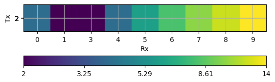
You can visualize the data in many ways depending on the physics manager. To simply view the data as a matrix you can use pg.viewer.mpl.showDataContainerAsMatrix. This visualizes a matrix of receivers and transmitters pairs with the associated data to plot : ‘dist’.
ax, cb = pg.viewer.mpl.showDataContainerAsMatrix(data, "Rx", "Tx", 'dist')
There are various formal methods for plotting different data containers, depending on the approach used. As discussed in Fundamentals, the primary focus here is on displaying the data container itself. Most method managers provide a .show() function specific to their method, but you can always use the main function pg.show(). This function automatically detects the data type and plots it accordingly. For further details on data visualization, please refer to Data visualization.