Modelling with Boundary Conditions

We use the preceding example (Poisson equation on the unit square) but want to specify different boundary conditions on the four sides.

Again, we first import numpy and pygimli, the solver and post processing functionality.

import numpy as np
import pygimli as pg

from pygimli.solver import solve
from pygimli.viewer import show
from pygimli.viewer.mpl import drawStreams

We create 21 x 21 node grid to solve on.

grid = pg.createGrid(x=np.linspace(-1.0, 1.0, 21),
                     y=np.linspace(-1.0, 1.0, 21))

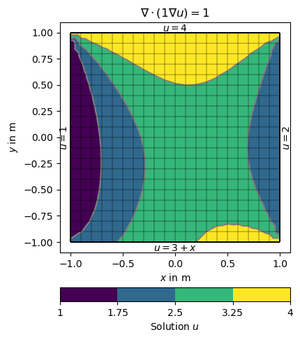
We start considering inhomogeneous Dirichlet boundary conditions (BC).

There are different ways of specifying BCs. They can be maps from markers to values, explicit functions or implicit (lambda) functions.

The boundary 1 (left) and 2 (right) are directly mapped to the values 1 and 2. On side 3 (top) a lambda function 3+x is used (p is the boundary position and p[0] its x coordinate. On side 4 (bottom) a function uDirichlet is used that simply returns 4 in this example but can compute anything as a function of the individual boundaries b.

def uDirichlet(boundary):
    """Return a solution value for a given boundary.
        Scalar values are applied to all nodes of the boundary."""
    return 4.0

dirichletBC = {1: 1,                                           # left
               2: 2.0,                                         # right
               3: lambda boundary: 3.0 + boundary.center()[0], # bottom
               4: uDirichlet}                                  # top

The boundary conditions are passed using the bc keyword dictionary.

u = solve(grid, f=1., bc={'Dirichlet': dirichletBC})

# Note that showMesh returns the created figure ax and the created colorBar.
ax, cbar = show(grid, data=u, label='Solution $u$')

show(grid, ax=ax)

ax.text(1.02, 0, '$u=2$', va='center', ha='left',  rotation='vertical')
ax.text(-1.01, 0, '$u=1$', va='center', ha='right', rotation='vertical')
ax.text(0, 1.01, '$u=4$', ha='center')
ax.text(0, -1.01, '$u=3+x$', ha='center', va='top')

ax.set_title('$\\nabla\cdot(1\\nabla u)=1$')

ax.set_xlim([-1.1, 1.1])  # some boundary for the text
ax.set_ylim([-1.1, 1.1])

(-1.1, 1.1)

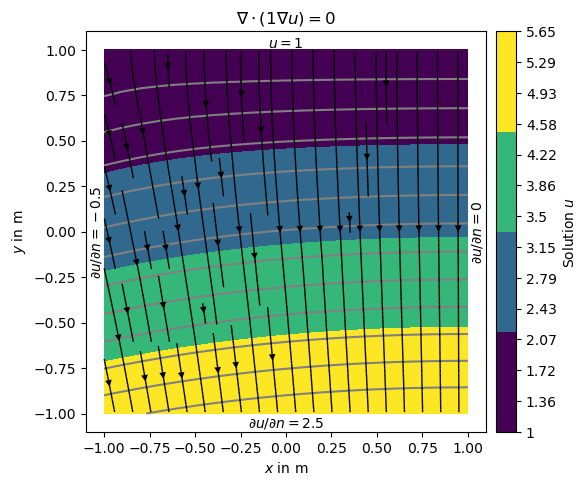
Alternatively we can define the gradients of the solution on the boundary, i.e., Neumann type BC. This is done with another dictionary {marker: value} and passed by the bc dictionary.

neumannBC = {1: -0.5,  # left
             4: 2.5}  # bottom

dirichletBC = {3: 1.0}  # top

u = solve(grid, f=0., bc={'Dirichlet': dirichletBC, 'Neumann': neumannBC})

Note that on boundary 2 (right) has no BC explicitly applied leading to default (natural) BC that are of homogeneous Neumann type \(\frac{\partial u}{\partial n}=0\)

ax = show(grid, data=u, filled=True, orientation='vertical',
          label='Solution $u$',
          levels=np.linspace(min(u), max(u), 14), hold=True)[0]

# Instead of the grid we now want to add streamlines to show the gradients of
# the solution (i.e., the flow direction).

drawStreams(ax, grid, u)

ax.text(0.0, 1.01, '$u=1$',
        horizontalalignment='center')  # top -- 3
ax.text(-1.0, 0.0, '$\partial u/\partial n=-0.5$',
        va='center', ha='right', rotation='vertical')  # left -- 1
ax.text(0.0, -1.01, '$\partial u/\partial n=2.5$',
        ha='center', va='top')  # bot -- 4
ax.text(1.01, 0.0, '$\partial u/\partial n=0$',
        va='center', ha='left', rotation='vertical')  # right -- 2

ax.set_title('$\\nabla\cdot(1\\nabla u)=0$')

ax.set_xlim([-1.1, 1.1])
ax.set_ylim([-1.1, 1.1])

(-1.1, 1.1)

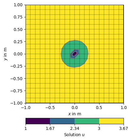
Its also possible to force single nodes to fixed values too. Short test: setting the value for the center node to 1.0

u = solve(grid, f=1., bc={'Node': [grid.findNearestNode([0.0, 0.0]), 1.0]})
np.testing.assert_approx_equal(u[grid.findNearestNode([0.0, 0.0])], 1.0, significant=10)

ax, _ = pg.show(grid, u, logScale=False, label='Solution $u$',)
_ = pg.show(grid, ax=ax)