Note
Go to the end to download the full example code.
The DataContainer class#
Data are often organized in a data container storing the individual data values as well as any description how they were obtained, e.g. the geometry of source and receivers.
So first a data container holds vectors like in a dictionary, however, all of them need to have the same length defined by the .size() method. Assume we want to store Vertical Electrical Sounding (VES) data.
# We start off with the typical imports
import numpy as np
import matplotlib.pyplot as plt
import pygimli as pg
from pygimli.physics import VESManager
We define logarithmically equidistant AB/2 spacings
ab2 = np.logspace(0, 3, 11)
print(ab2)
[   1.            1.99526231    3.98107171    7.94328235   15.84893192
   31.6227766    63.09573445  125.89254118  251.18864315  501.18723363
 1000.        ]
We create an empty data container
ves = pg.DataContainer()
print(ves)
Data: Sensors: 0 data: 0, nonzero entries: []
We feed it into the data container just like in a dictionary.
Data: Sensors: 0 data: 11, nonzero entries: ['ab2', 'mn2']
We now want to do a VES simulation and use the VES Manager for this task.
mgr = VESManager()
model = [10, 10, 100, 10, 1000]
ves["rhoa"] = mgr.simulate(model, ab2=ves["ab2"], mn2=ves["mn2"])
print(ves)
Data: Sensors: 0 data: 11, nonzero entries: ['ab2', 'mn2', 'rhoa']
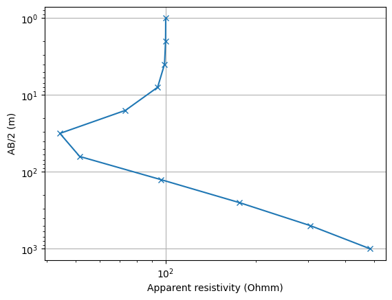
We can plot the sounding curve by assessing its fields
fig, ax = plt.subplots()
ax.loglog(ves["rhoa"], ves["ab2"], "x-");
ax.set_ylim(ax.get_ylim()[::-1])
ax.grid(True)
ax.set_xlabel("Apparent resistivity (Ohmm)")
ax.set_ylabel("AB/2 (m)");
Text(24.000000000000007, 0.5, 'AB/2 (m)')
A data container can be saved to disk
ves.save("ves.data")
print(open("ves.data").read())
0
# x y z
11
# ab2 mn2 rhoa valid
1.00000000000000e+00    3.33333333333333e-01    9.99842595368026e+01    0
1.99526231496888e+00    6.65087438322960e-01    9.98766666391267e+01    0
3.98107170553497e+00    1.32702390184499e+00    9.90710153790337e+01    0
7.94328234724281e+00    2.64776078241427e+00    9.39205974843448e+01    0
1.58489319246111e+01    5.28297730820371e+00    7.33018913900196e+01    0
3.16227766016838e+01    1.05409255338946e+01    4.41998154306538e+01    0
6.30957344480193e+01    2.10319114826731e+01    5.14873009414442e+01    0
1.25892541179417e+02    4.19641803931389e+01    9.61269991281245e+01    0
2.51188643150958e+02    8.37295477169860e+01    1.76491691336385e+02    0
5.01187233627272e+02    1.67062411209091e+02    3.05345771380821e+02    0
1.00000000000000e+03    3.33333333333333e+02    4.83494826609041e+02    0
0
The data are (along with a valid flat) in the second section. We can add arbitrary entries to the data container but define what to save.
ves["flag"] = pg.Vector(ves["rhoa"] > 100) + 1
print(ves)
ves.save("ves.data", "ab2 mn2 rhoa")
print(open("ves.data").read())
Data: Sensors: 0 data: 11, nonzero entries: ['ab2', 'flag', 'mn2', 'rhoa']
0
# x y z
0
# ab2 mn2 rhoa
0
We can mask or unmask the data with a boolean vector.
ves.markValid(ves["ab2"] > 2)
ves.save("ves.data", "ab2 rhoa")  # note that only valid data are saved!
print(ves)
Data: Sensors: 0 data: 11, nonzero entries: ['ab2', 'flag', 'mn2', 'rhoa', 'valid']
Data containers with indexed data#
Assume we have data associate with a transmitter, receivers and a property U. The transmitter (Tx) and receiver (Rx) positions are stored separately and we refer them with an Index (integer). Therefore we define these fields index.
data = pg.DataContainer()
data.registerSensorIndex("Tx")
data.registerSensorIndex("Rx")
print(data)
Data: Sensors: 0 data: 0, nonzero entries: ['Rx', 'Tx']
Create a list of 10 sensors, 2m spacing
Data: Sensors: 10 data: 0, nonzero entries: ['Rx', 'Tx']
We want to use all of them (and two more!) as receivers and a constant transmitter of number 2.
data["Rx"] = np.arange(12)
# data["Tx"] = np.arange(9) # does not work as size matters!
data["Tx"] = pg.Vector(data.size(), 2)
print(data)
data.save("TxRx.data")
print(open("TxRx.data").read())
Data: Sensors: 10 data: 12, nonzero entries: ['Rx', 'Tx']
10
# x y z
0       0       0
2       0       0
4       0       0
6       0       0
8       0       0
10      0       0
12      0       0
14      0       0
16      0       0
18      0       0
12
# Rx Tx valid
1       3       0
2       3       0
3       3       0
4       3       0
5       3       0
6       3       0
7       3       0
8       3       0
9       3       0
10      3       0
11      3       0
12      3       0
0
Again, we can mark the data validity.
data.markValid(data["Rx"] >= 0)
print(data["valid"])
print(data["Rx"])
12 [1.0, 1.0, 1.0, 1.0, 1.0, 1.0, 1.0, 1.0, 1.0, 1.0, 1.0, 1.0]
[ 0  1  2  3  4  5  6  7  8  9 10 11]
or check the data validity automatically.
data.checkDataValidity()
print(data["valid"])
data.removeInvalid()
print(data)
# data.save("TxRx.data");
10 [1.0, 1.0, 1.0, 1.0, 1.0, 1.0, 1.0, 1.0, 1.0, 1.0]
Data: Sensors: 10 data: 10, nonzero entries: ['Rx', 'Tx', 'valid']
Suppose we want to compute the horizontal offset between Tx and Rx. We first retrieve the x position and use Tx and Rx as indices.
10 [4.0, 2.0, 0.0, 2.0, 4.0, 6.0, 8.0, 10.0, 12.0, 14.0]
It might be useful to only use data where transmitter is not receiver.
data.markInvalid(data["Rx"] == data["Tx"])
print(data)
# data.save("TxRx.data");
Data: Sensors: 10 data: 10, nonzero entries: ['Rx', 'Tx', 'dist', 'valid']
They are still there but can be removed.
data.removeInvalid()
print(data)
Data: Sensors: 10 data: 9, nonzero entries: ['Rx', 'Tx', 'dist', 'valid']
At any stage we can create a new sensor
data.createSensor(data.sensors()[-1])
print(data)  # no change
Data: Sensors: 10 data: 9, nonzero entries: ['Rx', 'Tx', 'dist', 'valid']
, however, not at a position where already a sensor is
data.createSensor(data.sensors()[-1]+0.1)
print(data)
# data.save("TxRx.data")
Data: Sensors: 11 data: 9, nonzero entries: ['Rx', 'Tx', 'dist', 'valid']
Any DataContainer (indexed or not) can be visualized as matrix plot
pg.viewer.mpl.showDataContainerAsMatrix(data, "Rx", "Tx", "dist");
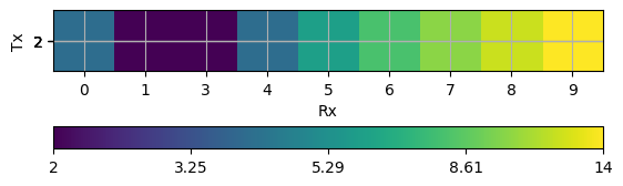
(<Axes: xlabel='Rx', ylabel='Tx'>, <matplotlib.colorbar.Colorbar object at 0x7fa649e21b50>)
Instead of marking and filtering one can remove directly
print(data["dist"])
data.remove(data["dist"] > 11)
print(data["dist"])
print(data)
9 [4.0, 2.0, 2.0, 4.0, 6.0, 8.0, 10.0, 12.0, 14.0]
7 [4.0, 2.0, 2.0, 4.0, 6.0, 8.0, 10.0]
Data: Sensors: 11 data: 7, nonzero entries: ['Rx', 'Tx', 'dist', 'valid']
Similar to the nodes of a mesh, the sensor positions can be changed.
data.scale([2, 1])
data.translate([10, 0])
data.save("TxRx.data")
1
Suppose a receiver has not been used
data["Rx"][5] = data["Rx"][4]
data.removeUnusedSensors()
print(data)
Data: Sensors: 8 data: 7, nonzero entries: ['Rx', 'Tx', 'dist', 'valid']
or any measurement with it (as Rx or Tx) is corrupted
data.removeSensorIdx(2)
print(data)
Data: Sensors: 0 data: 0, nonzero entries: ['Rx', 'Tx']
There are specialized data containers with predefined indices like pg.DataContainerERT having indices for a, b, m and b electrodes. One can also add alias translators like C1, C2, P1, P2, so that dataERT[“P1”] will return dataERT[“m”]