4. Meshes#
This part of the user guide covers mesh-related topics, starting with a general introduction to the mesh class. Moreover, this section introduces general operations to create or import meshes. The general aspects of visualization are covered in the visualization section.
4.1. Basics of the mesh class#
We start off by looking at the general anatomy of a pyGIMLi mesh. It is represented by a collection of nodes, cells and boundaries, i.e., geometrical entities:
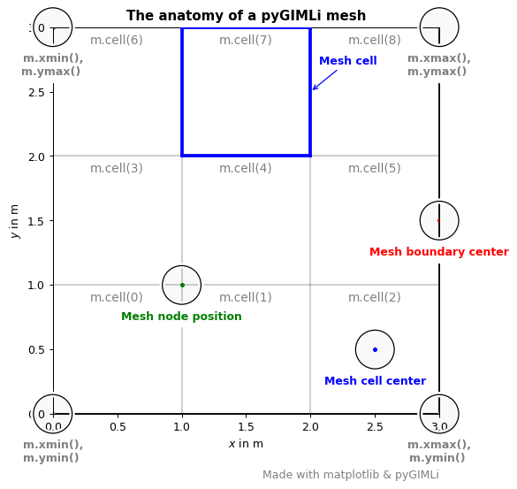
The mesh class holds either geometric definitions (piece-wise linear complex - PLC) or discretizations of the subsurface. It contains nodes, boundaries (edges in 2D, faces in 3D) and cells (triangles, quadrangles in 2D, hexahedra or tetrahedra in 3D) with associated markers and arbitrary data for nodes or cells.
Working with meshes
Function |
Usage |
|---|---|
|
Allows to access mesh cells |
|
Allows to access a single cell (using the cell ID) |
|
Allows to point to the center of a specific mesh cell |
|
Allows to extract the x / y coordinate of a cell center |
|
Accesses mesh boundaries |
|
Points to a specific boundary of the mesh (using boundary IDs) |
|
Allows to point to the center of a specific mesh boundary |
|
Allows to extract x / y coordinate of a boundary |
|
Accesses mesh nodes |
|
Refers to one specific node within the mesh |
|
Allows to extract x / y coordinate of a node |
It is common practice to classify meshes into two main types - structured and unstructured.
Structured meshes are meshes with implicit connectivit, exhibiting a well-known pattern in which the cells are arranged. As the cells are in a particular order, the topology of such mesh is regular. Such meshes enable easy identification of neighboring cells and points, because of their formation and structure. Often structured meshes have orthogonal quadrilateral (2D) or hexahedral (3D) elements.
Structured meshes
A regularly spaced mesh consisting of rectangles or hexahedrons is usually called a grid. However, a grid is just a special variant of a mesh so GIMLi treats it the same. The only difference is how they are created.
Unstructured meshes, as the name suggests, are more general and can randomly form any geometry shape. Unlike structured meshes, the connectivity pattern is not fixed hence unstructured meshes do not follow a uniform pattern. However, unstructured meshes are more flexible and thus allow for more complex applications.
from pygimli.meshtools import polytools as plc

fig, (ax1,ax2) = plt.subplots(1,2,figsize=(16,8), dpi=90)
ax1.set_title("Structured mesh", fontweight="bold")
ax2.set_title("Unstructured mesh", fontweight="bold")

# Create geometry
world = plc.createWorld(start=[-10, 0], end=[10, -10], marker=1,
                        worldMarker=False)
c1 = plc.createCircle(pos=[0.0, -5.0], radius=3.0, area=.3)

# Structured mesh
xmin, xmax = -10, 10.
zmin, zmax = -10., 0.

xreg = np.linspace(xmin, xmax, 20)
zreg = np.linspace(zmin, zmax, 10)
m_reg = pg.meshtools.createGrid(xreg,zreg,marker=2)

pg.show(m_reg, ax=ax1)
# Unstructured mesh
m = pg.meshtools.createMesh(world, quality=34, area=1)
pg.show(m, ax=ax2)
fig.tight_layout()

4.2. Mesh creation#
4.2.1. Creating a regular mesh / grid in 2D#
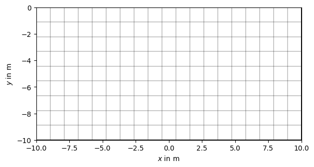
To create a regular 2D grid, pyGIMLi offers a variety of tools that help with the task. To create a regular grid, we first of all have to create the extent of the mesh in x and z direction. For this example, we create a mesh of 20 x 10 m with a regular cell size of 1 x 1 m. After defining the extent, we can simply call the pg.meshtools.createGrid() and get an overview of the number of nodes, cells and boundaries:
xmin, xmax = -10, 10.
zmin, zmax = -10., 0.

xreg = np.linspace(xmin, xmax, 20)
zreg = np.linspace(zmin, zmax, 10)
m_reg = pg.meshtools.createGrid(xreg,zreg,marker=2)
m_reg
Mesh: Nodes: 200 Cells: 171 Boundaries: 370
To show the mesh, we can simply call the pg.show() function:
pg.show(m_reg)
(<Axes: xlabel='$x$ in m', ylabel='$y$ in m'>, None)
Regular grids in 2D
Function |
Usage |
|---|---|
Creates a regular grid mesh from the provided x- and z-coordinates |
4.2.2. Creating an irregular mesh with pyGIMLi#
After covering the basics of regular grids, we want to dive into the world of irregular meshes.
However, we first of all have to create a geometry that is used as underlying susurface model for the mesh creation.
# dimensions of the world
left = -30
right = 30
depth = 25

world = mt.createWorld(start=[left, 0],
                       end=[right, -depth],
                       layers=[-5], worldMarker=False)
print(world)
pg.show(world)
Mesh: Nodes: 6 Cells: 0 Boundaries: 7
(<Axes: xlabel='$x$ in m', ylabel='$y$ in m'>, None)
Region markers
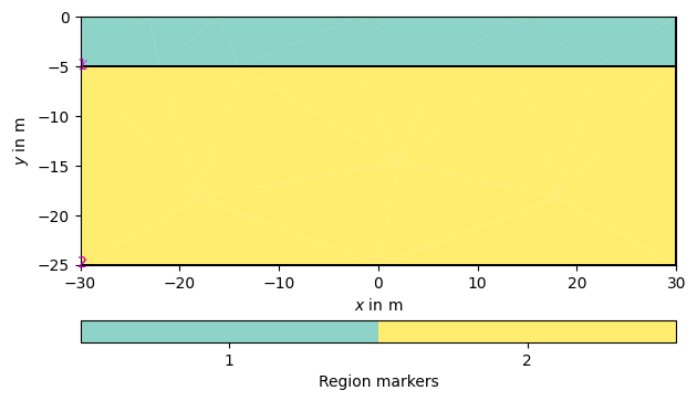
A mesh can have different regions, which are defined by region markers for each cell. Region markers can be used to assign properties for forward modelling as well as to control the inversion behavior.
For more information, see the later section on Markers
We are using the mt.createWorld() function to create a world based on the gíven x- & z-coordinates. The following table lists all handy functions that can be utilized when creating a geometry in pyGIMLi:
PLC creation in pyGIMLi
Function |
Usage |
|---|---|
Creates a PLC out of a given geometry |
|
Creates a circular PLC |
|
Creates a cubic PLC |
|
Creates a cylindric PLC |
|
Creates a line polygon |
|
Creates a polygon from a list of vertices |
|
Creates a rectangular PLC |
pyGIMLi has different ways to create meshes. mt.createMesh creates a mesh using Triangle, a two-dimensional constrained Delaunay mesh generator.
The additional input parameters control the maximum triangle area and the mesh smoothness. The quality factor prescribes the minimum angles allowed in the final mesh. This can improve numerical accuracy, however, fine meshes lead to increased computational costs. Notice that we are now using showMesh which is convenient for 2D mesh visualization.
from pygimli.viewer import showMesh

mesh = mt.createMesh(world,
                     area=2.0,
                     quality=33,
                     smooth=[2, 4] # [0:no smoothing or 1:node center or 2:weighted node center, # of iter]
                    )
showMesh(mesh, markers=True, showMesh=True);

4.3. Utilizing markers#
A mesh can have different regions, which are defined by region markers for each cell. Region markers can be used to assign properties for forward modelling as well as to control the inversion behavior. Moreover, a pyGIMLi mesh holds specific markers for all boundaries (outer mesh boundaries as well as interfaces between layers and boundaries around structures, see figure above). Those boundary markers are used to define specific properties or conditions on the boundaries of a mesh. They are essential for setting up boundary conditions in simulations, such as specifying fixed values or fluxes. Properly assigning boundary markers ensures accurate representation of physical boundaries and interactions in the model.
When constructing complex geometries out of basic geometric shapes (e.g., circle, rectangle, …) we need to be careful with both the region and boundary markers. In this user guide, we explain the differences as well as the usage of both types of markers.
4.3.1. Region markers#
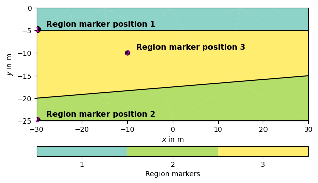
Let’s take a closer look at the region markers of the two-layer case presented above. Every region marker of a specific mesh region has a position, which it is assigned to. By using ``, we can visualize the position in the PLC:
fig, ax = plt.subplots(1,1)
pg.show(world, ax=ax)
for nr, marker in enumerate(world.regionMarkers()):
    print('Position marker number {}:'.format(nr + 1), marker.x(), marker.y(),
          marker.z())
    ax.text(marker.x()+2,marker.y()+2, f"Region marker position {nr+1}",
            fontweight="bold",fontsize=11, ha="left", va="top", color="black")
    ax.scatter(marker.x(), marker.y(), s=(4 - nr) * 20, color='k')
Position marker number 1: -29.8 -4.8 0.0
Position marker number 2: -29.8 -24.8 0.0
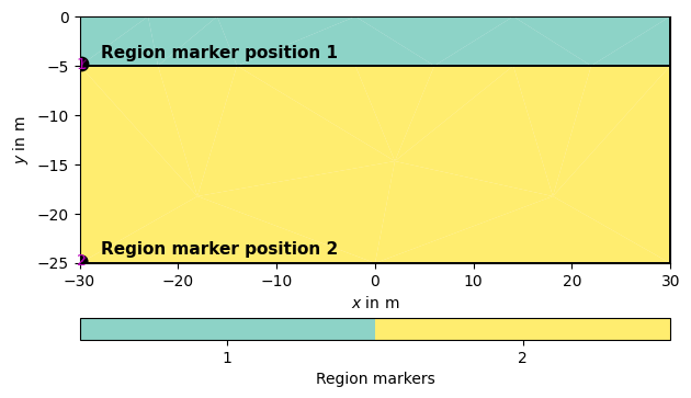
By default, pyGIMLi assigns unique markers to every region of the PLC, starting from 1. A marker value of 0 is assigned to a region if no region marker is found - but even if this happens, we could still manually add a marker to the specific region. For now, we want to add a polygon to the already existing 2-layer PLC. This is done using the createPolygon() function. Within this function, we have two adjusting variables for the region markers - marker and markerPosition. The first variable specifies the marker number and the second the position of the marker. Note, that the position of a region marker has to lie within its region to work! In this case, we specify the newly defined region to have the marker 3. The marker position is set to [-10, -10].
poly = mt.createPolygon([[left, -20], [right,-15],[right,-5],[left,-5]], isClosed=True, marker=3, markerPosition=[-10, -10])
geometry = world + poly
fig, ax = plt.subplots(1,1)
pg.show(geometry, ax=ax)
for nr, marker in enumerate(geometry.regionMarkers()):
    print('Position marker number {}:'.format(nr + 1), marker.x(), marker.y(),
          marker.z())
    ax.text(marker.x()+2,marker.y()+2, f"Region marker position {nr+1}",
            fontweight="bold",fontsize=11, ha="left", va="top", color="black")
    ax.scatter(marker.x(), marker.y(), s=(4 - nr) * 20, color='k')
Position marker number 1: -29.8 -4.8 0.0
Position marker number 2: -29.8 -24.8 0.0
Position marker number 3: -10.0 -10.0 0.0
Of course it is also possible to assign the same region marker to multiple parts of your PLC. This gets especially handy as soon as you start assigning physical parameters to your meshed geometry for modelling and/or inversion purposes. For more detailed information on this matter, please take a look at the modelling section of the user guide.
4.3.2. Boundary markers#
If we talk about markers in a PLC, one often forgets about the boundary markers. If you create a geometry in pyGIMLi, no matter whether it is a circle, rectangle or layered world, you need to deal with boundaries of different kinds. pyGIMLi automatically assigns numbers to the boundaries and, doing so, follows a specific pattern. In order to change the default boundary markers, please refer to the modelling section of the user guide.
If we assume a simple rectangular world without additional layers, we have two different options on how to enumerate the boundaries:
Set
createWorld(worldMarker=False), which leads to enumerated boundaries (1 = left, 2=right, 3=bottom, 4=top, 5=front and 6=back).Set
createWorld(worldMarker=True), which leads to the top holding the boundary marker -1 and other outer boundaries -2.
start = [left,0]
end = [right, -depth]
world1 = mt.createWorld(start=start,
                       end=end, worldMarker=False)

world2 = mt.createWorld(start=start,
                       end=end, worldMarker=True)

fig, (ax1,ax2) = plt.subplots(1,2,figsize=(16,12), dpi=90)
ax1.set_title("worldMarker = False", fontweight="bold")
ax2.set_title("worldMarker = True", fontweight="bold")

pg.show(world1, markers=True, ax=ax1)
pg.show(world2, markers=True, ax=ax2)
(<Axes: title={'center': 'worldMarker = True'}, xlabel='$x$ in m', ylabel='Depth in m'>,
 None)

Let’s assume that we want to add an additional feature to our PLC, such as a rectangle. Doing so, the circle is automatically assigned a boundary marker - in this case 1. However, assuming the case where we set worldMarker=False, this marker is already assigned to the left boundary of the PLC (which could cause problems in any modelling application later on). So we need to adapt the boundary marker of the circle, which is simply done as follows:
c1 = plc.createRectangle(start=[-10,-5], end=[10,-10], marker=2)
geom1 = world1+c1
# %%
for i in range(geom1.boundaryCount()):
    if i >= 4:
        geom1.boundary(i).setMarker(5)

pg.show(geom1, markers=True)
(<Axes: xlabel='$x$ in m', ylabel='$y$ in m'>, None)
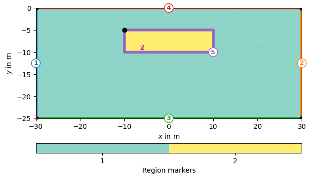
As you can see, the boundaries around the rectangle were all changed to 5, as defined in the for-loop above. PLC.boundaryCount() gives us the total count of boundaries in the PLC, while PLC.boundary().setMarker() allows us to change a specific boundary marker.
To see applications where the indices of the PLC / mesh boundary are utilized, please refer to the modelling section of the user guide.
4.4. Mesh import#
4.4.1. Import options for meshes in pyGIMLi#
A broad variety of functions to import and convert different mesh types into a GIMLI mesh object exists within pyGIMLi. The following functions are the most commonly used ones:
PLC creation in pyGIMLi
Function |
Usage |
|---|---|
Read FEniCS mesh from .h5 format and return a GIMLI mesh object |
|
Read GMSH ASCII file and return a GIMLI mesh object |
|
Load a mesh from HDF5 file format |
|
Import mesh from Hydrus 2D |
|
Import mesh from Hydrus 3D |
|
Read generic meshIO mesh |
|
Read STL surface mesh and converts to GIMLI mesh object |
|
Read and convert a mesh from the basic Tetgen output |
|
Read Triangle mesh |
4.4.2. Example: mesh generation using Gmsh#
When the scientific task requires a complex finite-element discretization (i.e. incorporation of structural information, usage of a complete electrode model (CEM), etc.), external meshing tools with visualization capabilities may be the option of choice for some users. In general, the bindings provided by pygimli allow to interface any external mesh generation software. For examples on how to use external meshing software, refer to the examples section on the pyGIMLi website.
4.5. Mesh modification#
pyGIMLi provides a variety of operators to modify your mesh. The following table gives an overview of the most important functions:
Mesh modifications
Function |
Usage |
|---|---|
Merges two meshes |
|
Merges two or more meshes |
|
|
Allows to translate a mesh |
|
Scale a mesh with provided factors |
|
Rotate a provided mesh |
4.5.1. Merging meshes#
In some cases, the modelling domain may require different degrees of flexibility in separate mesh regions. In the following, we demonstrate this for a two-dimensional mesh consisting of a region with regularly spaced quadrilaterals and a region with unstructured triangles.
pyGIMLi offers the possibility to merge two meshes by calling merge2Meshes.
xmin, xmax = -30, 30.
zmin, zmax = -50, -25.

xreg = np.linspace(xmin, xmax, 30)
zreg = np.linspace(zmin, zmax, 25)

mesh2merge = mt.createGrid(xreg, zreg, marker=3)
mergedMesh = mt.merge2Meshes(mesh,mesh2merge)
pg.show(mergedMesh, markers=True, showMesh=True)
(<Axes: xlabel='$x$ in m', ylabel='$y$ in m'>,
 <matplotlib.colorbar.Colorbar at 0x14c691ffeb90>)
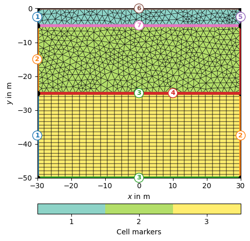
The merged meshes appear as a singular hybrid mesh now, so we can append a triangle boundary as for non-hybrid meshes:
mesh_append = mt.appendTriangleBoundary(mergedMesh, xbound=50., ybound=50., quality=31, smooth=True,
                                 marker=4, isSubSurface=True, addNodes=10)

ax, cb = pg.show(mesh_append)
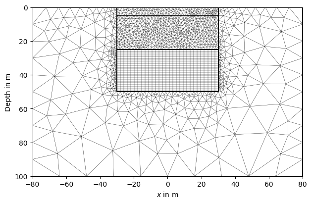
When merging more than two meshes, the function mergeMeshes() can be utilized instead of merge2Meshes.
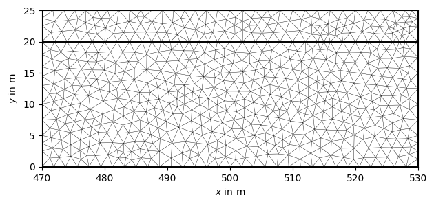
4.5.2. Translating meshes#
To perform simple changes of the meshs x- and z-coordinates, we can make use of the translate function. The following lines of code move the mesh 500 m in x and 25 m in z direction:
translated_mesh = pg.Mesh(mesh)
translated_mesh.translate([500, 25])
pg.show(translated_mesh)
(<Axes: xlabel='$x$ in m', ylabel='$y$ in m'>, None)
4.5.3. Scaling meshes#
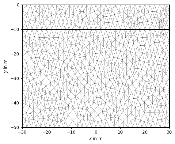
Apart from moving the mesh along its axes, pyGIMLi also provides a tool to scale the mesh along specified axes - in this example, we scale along the z-axis with a factor of 2:
scaled_mesh = pg.Mesh(mesh)
scaled_mesh.scale([1, 2])
pg.show(scaled_mesh)
(<Axes: xlabel='$x$ in m', ylabel='$y$ in m'>, None)
4.5.4. Rotating meshes#
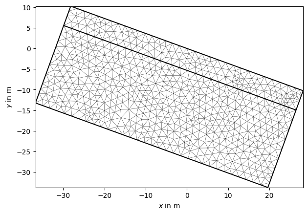
Another valuable mesh modification tool is the mesh.rotate function. By providing a rotation angle and the rotation plane, we can adjust the orientation angle of our mesh:
import numpy as np
rotated_mesh = pg.Mesh(mesh)
rotated_mesh.rotate([0, 0, np.deg2rad(-20)])
pg.show(rotated_mesh)
(<Axes: xlabel='$x$ in m', ylabel='$y$ in m'>, None)
4.6. Mesh export#
Suppose we want to continue working on our GIMLi mesh object in a different meshing tool - pyGIMLi provides a variety of export functions to transfer your GIMLi mesh into a different format:
Mesh export functions
Function |
Usage |
|---|---|
Exports GIMLi mesh in HDF5 format suitable for Fenics |
|
Writes given GIMLI::Mesh in a hdf5 format file |
|
Export a piece-wise linear complex (PLC) to a .poly file (2D or 3D) |
|
Write STL surface mesh |
|
|
Save mesh alongside properties as vtk |
# Save rotated mesh from above as vtk file

rotated_mesh.exportVTK('rotated_mesh.vtk')