5. Inversion#
5.1. Theory#
Inversion frameworks are generalized, abstract approaches to solve a specific inversion problem without specifying the appropriate geophysical methods. This can be a specific regularization strategy, an alternative formulation of the inverse problem or algorithms of routine inversion. It is initialized by specific forward operators or managers that provide them.
5.1.1. The objective function#
For all inversion frameworks the minimization of an objective function is required. The most common approaches are based on least-squares minimization of a data misfit term between the individual data \(d_i\) and the corresponding forwarc response \(f_i(\mathbf{m})\) of the model \(\mathbf{m})\). In order to account for measuring errors, we weight the residuals with the inverse of the error \(\epsilon_i\) so that the overall data objective function \(\Phi_\text{d}\) reads:
where \(\mathbf{W}_\text{d}\) is the data weighting matrix containing the inverse data errors and \(\mathbf{\mathcal{F}}(\mathbf{m})\) is the forward response vector for the model \(\mathbf{m}\). As the forward operator is in general non-linear, the minimization of the data misfit term requires iterative linearization approaches, starting from an initial model \(\mathbf{m}^0\) and updating the model in each iteration \(k\) by \(\Delta \mathbf{m}^k\):
The step length \(\tau^k\) can be determined by line search strategies to ensure sufficient decrease of the objective function in each iteration.
For inversion of a limited number of parameters (e.g., 1D layer models, spectral parameters) the minimization is performed solely based on the data (\(\Phi_d\rightarrow\min\)) by some stabilizing damping terms, as with the Levenberg-Marquardt [Levenberg, 1944, Marquardt, 1963] method. However, for large-scale problems (e.g., 2D/3D mesh-based inversion) the direct minimization is often not feasible.
5.1.2. Regularization#
To stabilize the inversion of ill-posed geophysical problems, additional constraints on the model parameters are required. A common approach is to add a regularization term \(\Phi_\text{m}\) to the objective function that penalizes undesirable model features. A very common choice for 2D/3D problems is the roughness of the model distribution, but there is a wide range of different regularization methods (different kinds of smoothness and damping, mixed operators, anisotropic smoothing). We express this term by the matrix \(\mathbf{W}_\text{m}\) acting on the model parameters \(\mathbf{m}\) and possibly a reference model \(\mathbf{m_0}\):
The dimensionless factor \(\lambda\) scales the influence of the regularization term \(\Phi_\text{m}\) (model objective function).
5.1.3. Minimization#
For minimizing the total objective function \(\Phi\), there are different available strategies:
Steepest-descent methods
Conjugate-gradient methods
Gauss-Newton methods
Quasi-Newton methods
Stochastic methods (e.g., genetic algorithms, Markov-Chain Monte Carlo)
5.1.3.1. Gradient-based methods#
An improvement is sought in the direction where \(\Phi\) descents most, i.e. the negative gradient \(-\mathbf{g}(m^k)=-\nabla_m \Phi=-\{\frac{\partial\Phi}{\partial m^k_i}\}\) is uses as model update direction \(\Delta\mathbf{m^k}\). Note that, assuming \(\Phi_d\) (and by the choice of \(\lambda\), \(\Phi_m\) likewise) is dimensionless, the choice of \(\tau^k\) depends on the model and is therefore crucial.
The gradient of the data objective function \(\Phi_d\) can be computed by
where the matrix \(\mathbf{J}\) is the Jacobian (also named sensitivity, see transforms below) matrix holding the derivatives of the forward computation with respect to the model parameters
In most cases, it can be computed without explicitly forming the Jacobian matrix. The gradient of the model objective function \(\Phi_m\) is
and therefore the gradient of \(\Phi\) calculates \(\mathbf{g}=\mathbf{g}_d+\lambda \mathbf{g}_m\).
This procedure defines the steepest-descent method, which is, however, known to be a slowly converging method.
The method is available under pygimli.frameworks.DescentInversion.
In the non-linear conjugate-gradient (NLCG) method, the model update directions are conjugated (i.e., they are pair-wise orthogonal) which speeds up the convergence a lot.
The method is available under pygimli.frameworks.NLCGInversion.
Both methods require the multiplication with the (transposed) sensitivity matrix, for which by default the Jacobian matrix is used, unless the function fop.STy() is implemented in the forward operator.
5.1.4. Newton-type methods#
5.1.4.1. Gauss-Newton method#
The default inversion framework is based on the generalized Gauss-Newton minimization scheme leading to the model update \(\Delta\mathbf{m}^k\) in the \(k^\text{th}\) iteration [Park and Van, 1991]:
with \(\Delta \mathbf{d}^k = \mathbf{d} − \mathcal{F}(\mathbf{m}^k)\) so that the new model is obtained by
The system of equations is solved using a conjugate-gradient based least-squares solver called CGLSCDPWW [Günther et al., 2006]. This solver also allows for flexible data and model parameters. For instance, as model parameters mostly represent (petro)physical properties, we use logarithmic parameters by default, but there is a wide range of transformations available, e.g. to bound the model parameters within plausible limits. This is all integrated in the inverse solver, i.e. the inner derivatives are computed on-the-fly. Therefore we differentiate between the Jacobian matrix of the forward operator using intrinsic properties like conductivity as input or apparent resistivity as output, also referred to as sensitivity matrix, and the Jacobian matrix of the inverse problem using transformed model and data parameters.
5.1.5. Transformations#
The inversion uses the term model \(m\), data \(d\) and a forward response \(f(m)\) as they might be implemented in a forward operator, e.g. resistivity or apparent resistivity. For reasons of stability and parameter tuning, one often applies certain transformation of the intrinsic readings \(r\) and model parameters \(p\). A very common choice is to use logarithmic parameters, i.e., \(m=\log p\), to ensure positive values for \(p\) (any \(m\) leads to \(p=\exp(m)\gt 0\)). One can also use a different lower boundary \(p_l\) so that \(m=\log(p-p_l)\) or an upper boundary \(p_u\) so that \(m=\log(p_u-p)\), both can be combined by \(m=\log(p-p_l)-\log(p_u-p)=\log\frac{p-p_l}{p_u-p}\), alternatively using a cotangens function \(m=-\cot\frac{p-p_l}{p_u-p}\pi\).
Similar transformations can be used for the data. As their choice is done in inversion and therefore independent on the forward operator, we distinguish the terms sensitivity (of the forward operators intrinsic parameters) \(S_{i,j}=\frac{\partial r}{\partial p}\) and the Jacobian using \(m\) and \(d\), which is computed as
5.1.6. Running inversion#
We will exemplify this by using a 1D Occam-style (smoothness constrained) inversion of vertical electric sounding (VES) data. We define a synthetic block model and compute a forward model for log-spaced AB/2 distances and use a forward operator with predefinied, log-equidistant thickness.
from pygimli.physics import ves
ab2 = np.logspace(0, 2.5, 21)
synth = [10, 10, 100, 300, 30]
data = ves.VESModelling(ab2=ab2).response(synth)
data *= (np.random.randn(len(data))*0.03 + 1)
thk = np.logspace(0, 1.8, 23)
fop = ves.VESRhoModelling(ab2=ab2, thk=thk)
24/03/26 - 14:06:33 - pyGIMLi - INFO - Found 1 regions.
We set up a simple inversion instance
inv = pg.Inversion(fop=fop)
inv.dataTrans = 'log' # inv.modelTrans is 'log' by default
m0 = inv.run(data, 0.02, startModel=100, maxIter=0, verbose=True)
24/03/26 - 14:06:33 - pyGIMLi - INFO - Starting inversion.
24/03/26 - 14:06:33 - pyGIMLi - INFO - fop: <pygimli.physics.ves.vesModelling.VESRhoModelling object at 0x14c01f9c88b0>
24/03/26 - 14:06:33 - pyGIMLi - INFO - Data transformation: Logarithmic transform
24/03/26 - 14:06:33 - pyGIMLi - INFO - Model transformation: Logarithmic transform
24/03/26 - 14:06:33 - pyGIMLi - INFO - min/max (data): 30.42/125
24/03/26 - 14:06:33 - pyGIMLi - INFO - min/max (error): 2%/2%
24/03/26 - 14:06:33 - pyGIMLi - INFO - min/max (start model): 100/100
min/max(dweight) = 50/50
--------------------------------------------------------------------------------
min/max(dweight) = 50/50
Building constraints matrix
constraint matrix of size(nBounds x nModel) 23 x 24
check Jacobian: wrong dimensions: (0x0) should be (21x24)  force: 1
jacobian size invalid, forced recalc: 1
24/03/26 - 14:06:34 - pyGIMLi - INFO - inv.iter 0 ... chi² = 568.94
Calculating Jacobian matrix (forced=1)...Create Jacobian matrix (brute force) ... ... 0.527455 s.
... 0.547524 s
min data = 30.4227 max data = 125.298 (21)
min error = 0.02 max error = 0.02 (21)
min response = 100 max response = 100 (21)
calc without reference model
0: rms/rrms(data, response) = 31.2199/83.1047%
0: chi^2(data, response, error, log) = 568.938
0: Phi = 11947.7 + 0 * 20 = 11947.7
and obtain a homogeneous model vector of 100 Ohmm.
At the beginning, \(\Phi_m=0\) and \(\mathbf{g}_m\) likewise.
The data residual inv.residual() drives the inversion.
Let’s do a gradient inversion step by hand:
dm0 = -inv.dataGradient() # equals -inv.gradient()
inv.model = np.exp(dm0)*inv.model
inv.response = fop(inv.model)
print(inv.chi2())
fig, ax = plt.subplots()
pg.viewer.mpl.drawModel1D(ax, model=synth, plot='loglog')
pg.viewer.mpl.drawModel1D(ax, thk, inv.model)
ax.invert_yaxis()
303.31418148509385
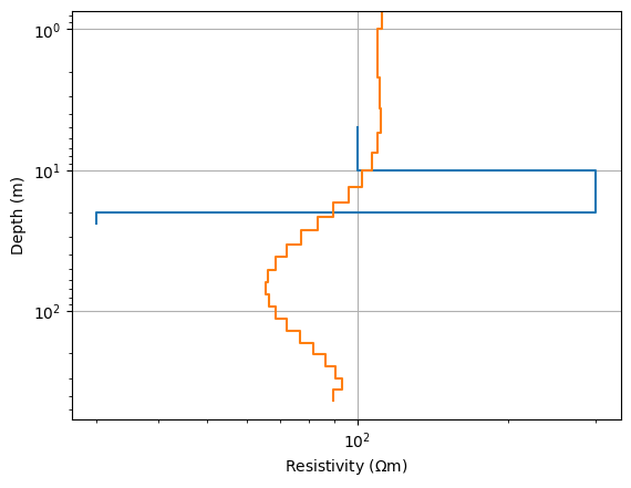
Note that usually inv.model and inv.response are updated by the minimization framework, but here we have to take the log-transformation into account.
The model shows an increase in the upper part and a decrease in the lower part.
The chi-square misfit has already reduced a fair amount.
Now we go one step further and compute another gradient, both for the data part and the model part, the first one wants to further decrease the data misfit and the second wants to get rid of the existing roughness in the model. We assume a regularization strength balancing those two of \(\lambda\)=10.
dg = -inv.dataGradient()
lam = 3
mg = -inv.modelGradient() * lam
ax, _ = pg.viewer.mpl.showModel1D(thk, inv.model, plot='loglog', label="model")
pg.viewer.mpl.drawModel1D(ax, model=synth, label="synth", color="black")
pg.viewer.mpl.drawModel1D(ax, thk, np.exp(dg)*inv.model, label="dataGradient")
pg.viewer.mpl.drawModel1D(ax, thk, np.exp(mg)*inv.model, label="modelGradient")
pg.viewer.mpl.drawModel1D(ax, thk, np.exp(mg+dg)*inv.model, ls="--", label="gradient")
ax.legend()
<matplotlib.legend.Legend at 0x14c01d324310>
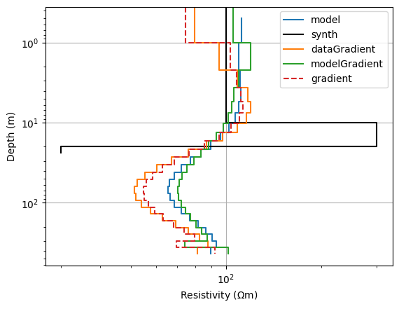
Whereas the model gradient tries to turn back the model to the homogeneous case, the data gradient wants to further exaggerate the anomaly. Combining both results in a trade-off that is closer to the latter, i.e. the larger data misfit (still) dominates. We finally update the model, but now we want to optimize the step length
from pygimli.frameworks import lineSearch
tau, resp = lineSearch(inv, mg+dg, method="quad", show=True)
print(tau)
newmodel = np.exp((mg+dg)*tau) * inv.model
newresponse = fop(newmodel)
print(inv.chi2(newresponse))
0.9249542951357778
235.5530777530908
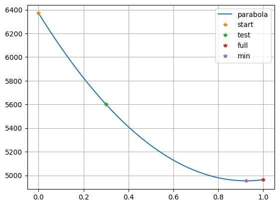
which fits a parabola through the old point (\(\tau\)=0), the full step (\(\tau\)=1) and a test (\(\tau\)=0.3) and obtain an optimum line search parameter of about 0.6-0.65.
As method, we can also use 'exact' (forward calculations) or 'inter' (interpolation), yielding almost the same results.
The latter is the simplest one and the former takes the most effort.
In total, the chi-square misfit, computed by \(\Phi_d/N\), decreases slowly.
As gradient-based minimization converges much slower, we switch to a Gauss-Newton framework.
After initialization, we set the model transformations as strings (we can also create instances)
We can choose lin, log, logL (L being lower bound), logL-U (two bounds), cotL-U or symlogT (T being the linear threshold).
The model roughness vector (including model transformation and weighting) can be
accessed by inv.roughness().
from pygimli.frameworks.inversion import GaussNewtonInversion

inv = GaussNewtonInversion(fop=fop)
inv.modelTrans = 'log' # already default
inv.dataTrans = 'log' # default linear
Like the transformations, there are a lot of options that can be set directly to the inversion instance:
fop- the forward operatorrobustData,blockyModel- use L1 norm for data misfit and model roughnessverbose- to see some outputmodel- the current modelresponse- the model responsedataVals,errorVals- data and error vectors
Most of them can also be passed to the inversion run and should better
maxIter- maximum iteration numberlam- the overall regularization strengthzWeight- the vertical-to-horizontal regularization ratio (2D/3D problems)startModel- the starting model as float or arrayrelativeErrorandabsoluteErrorto define the error modellimits- list of lower and upper parameter limits (overridinginv.modelTrans)
After running the inversion
model = inv.run(data, relativeError=0.03, verbose=True)
24/03/26 - 14:06:35 - pyGIMLi - INFO - Starting inversion.
24/03/26 - 14:06:35 - pyGIMLi - INFO - fop: <pygimli.physics.ves.vesModelling.VESRhoModelling object at 0x14c01f9c88b0>
24/03/26 - 14:06:35 - pyGIMLi - INFO - Data transformation: Logarithmic transform
24/03/26 - 14:06:35 - pyGIMLi - INFO - Model transformation: Logarithmic transform
24/03/26 - 14:06:35 - pyGIMLi - INFO - min/max (data): 30.42/125
24/03/26 - 14:06:35 - pyGIMLi - INFO - min/max (error): 3%/3%
24/03/26 - 14:06:35 - pyGIMLi - INFO - My model 24 [102.84353794128707, 102.84353794128707, 102.84353794128707, 102.84353794128707, 102.84353794128707, 102.84353794128707, 102.84353794128707, 102.84353794128707, 102.84353794128707, 102.84353794128707, 102.84353794128707, 102.84353794128707, 102.84353794128707, 102.84353794128707, 102.84353794128707, 102.84353794128707, 102.84353794128707, 102.84353794128707, 102.84353794128707, 102.84353794128707, 102.84353794128707, 102.84353794128707, 102.84353794128707, 102.84353794128707]
24/03/26 - 14:06:35 - pyGIMLi - INFO - inv.iter 0 ... chi² = 264.53
--------------------------------------------------------------------------------
--------------------------------------------------------------------------------
inv.iter 1 ...
24/03/26 - 14:06:35 - pyGIMLi - INFO - tau: 0.901
24/03/26 - 14:06:35 - pyGIMLi - INFO - chi² = 2.01 (dPhi = 98.89%) lam: 20.0
Create Jacobian matrix (brute force) ... ... 0.545175 s.
--------------------------------------------------------------------------------
inv.iter 2 ...
24/03/26 - 14:06:36 - pyGIMLi - INFO - tau: 1.0
24/03/26 - 14:06:36 - pyGIMLi - INFO - chi² = 0.81 (dPhi = 45.44%) lam: 20.0
24/03/26 - 14:06:36 - pyGIMLi - INFO -
Create Jacobian matrix (brute force) ... ... 0.509027 s.
################################################################################
#                  Abort criterion reached: chi² <= 1 (0.81)                   #
################################################################################
we observe that the data are fitted within noise in very few iterations.
The chi-square value can be accessed by inv.chi2(), its convergence is stored in
inv.chi2History. The data, model and total objective function values can be retrieved
by inv.phiData(), inv.phiModel() and inv.phi(). By default, the current model and
its response are used, alternatively you can pass model= to phiModel() or phi()
and response= to phiData() and phi().
The important measure of data fit is the chi-square value
as it includes the error model (and the data transformation). In many cases, one has a better feeling by computing the (untransformed) root-mean-square (RMS), either absolute
by using inv.absrms(), or relative
by using inv.relrms().
Traveltime tomography is a good example for looking at ARMS (e.g. in ms), while in ERT
one usually has a good feeling for RRMS (same for voltage, resistance or apparent
resistivity) in %.
5.1.7. Error model and misfit#
One needs to distinguish between the actual data errors (unknown random values) and the error model, an assumption of the standard deviation of the individual data. Note that this reflects our expectation on how well we can fit the data. A standard deviation from repeated measurements helps to detect outliers and to get a rough idea of an error model, but often underestimates the real errors.
The error model plays a crucial role in the inversion process as it weights the data against each other and data and model objective function. In case the errors are known, the regularization strength \(\lambda\) needs to be chosen so that the mean squared data misfit \(\chi^2\) reaches a value of about 1, indicating that the data are explained within their errors. To this end, the regularization strength should be adjusted so that, according to Occams razor principle, the simplest model explaining the data within their errors is found. In many cases, simple means smooth, so that the smoothest model reaching \(\chi^2\approx 1\) is sought.
However, one can adapt the regularization in a way that the meaning of simple reflects the prior knowledge or assumption about the subsurface. This could be different weights for horizontal and vertical smoothness, spatially varying regularization etc.
We expect the data misfit (\((\mathbf{d}-\mathbf{f}(\mathbf{m}))/\epsilon\) including data
transformation), that can be retrieved by inv.residual(), to contain only random noise,
i.e., a normal distribution with zero mean and standard deviation of 1 (\(\chi^2=1\)).
So one should have a look at both the histogram and the distribution (e.g. plotting like
a sounding curve) of the misfit to ensure it contains uncorrelated Gaussian noise.
If there are outliers in the histogram, one can eliminate them.
If there are systematic effects (“structure in the misfit”), one could probably reduce
the error model.
5.1.8. Model appraisal#
A necessary, but not sufficient condition for resolving an anomaly in the subsurface is that the data are sensitive to changes in the model parameters at the corresponding position.
For all minimization types, we can access the Jacobian matrix (different matrix types) by
inv.jacobianMatrix(error_weighted=False, numpy_matrix=False), optionally error-weighted
or converted to numpy.
The overall sensitivity of the model can be obtained by summing up the absolute values of the sensitivity matrix (Jacobian) rows. In analogy to the total ray length in traveltime tomography it is also referred to as coverage.
A high coverage does not guarantee high resolution, e.g., the same measurement can be done several times or very similar measurements are performed, so we need a certain degree of independence of the data to resolve model parameters.
However, e.g., [Ronczka et al., 2017] showed that the coverage can be used as a rough estimate of resolution radius, which requires higher computational effort. Therefore, the coverage can be used for alpha-shading of the model, or for thresholding the well-resolved model parts.
More correctly, one can have a look at the formal resolution matrices to retrieve uncertainty, resolution radii or information content used for experimental design [Wagner et al., 2015]. For details we refer to [Günther, 2004]. We plot both matrices for our case.
from pygimli.frameworks.resolution import resolutionMatrix
RM, RD = resolutionMatrix(inv, returnRD=True)
fig, ax = plt.subplots(ncols=2)
ax[0].imshow(RM, vmin=-1, vmax=1, cmap="bwr")
ax[1].imshow(RD, vmin=-1, vmax=1, cmap="bwr")
ax[0].set_title("RM")
ax[1].set_title("RD")
Text(0.5, 1.0, 'RD')
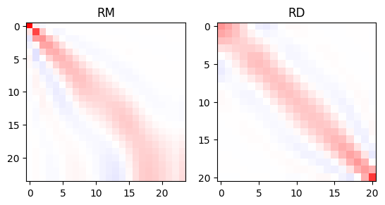
The resolution power of the individual layers decreases with depth, except the very last layer that is better determined. The data resolution matrix tells us about the importance of individual data and how they are related to each other. In our case the overall importance is highest for the smallest and biggest AB/2, and there is a large correlation between neighboring AB/2.
From the model resolution matrix, one can also compute a resolution radius [Friedel, 2003].
rm = np.diag(RM)
print(thk/rm[:-1])
[  1.03026214   1.6568211    3.47230476   4.96653449   6.75570299
   8.92284914  11.68718908  14.96869267  19.49922027  26.8901614
  37.79682081  49.97577147  58.44022799  61.89541953  67.03218854
  82.3222293  111.88924806 149.4513469  188.2505033  240.79369502
 333.35087962 506.97669295 838.62379155]
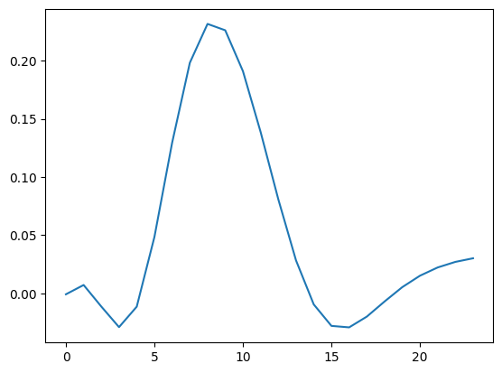
For large inverse problems, is it prohibitive to compute the whole matrix \(R_M\), but one can retrieve individual rows, referred to as resolution kernels, as, e.g., been used by [Rochlitz et al., 2025].
from pygimli.frameworks.resolution import modelResolutionKernel
rm8 = modelResolutionKernel(inv, 8)
plt.plot(rm8)
[<matplotlib.lines.Line2D at 0x14c01cf9b510>]
5.1.9. Frameworks#
Beyond different inversion approaches there are so-called frameworks for typical inversion (mostly regularization) tasks. Examples that are already implemented in pyGIMLi are for example:
Marquardt scheme inversion of few independent parameters, e.g., fitting of spectra [Loewer et al., 2017]
Soil-physical model reduction incorporating soil-physical functions [Costabel and Günther, 2014, Igel et al., 2016]
Classical joint inversion of two data sets for the same parameter like DC and EM [Günther, 2013]
Block joint inversion of several 1D data using common layers, e.g., MRS+VES [Günther and Müller-Petke, 2012]
Sequential (constrained) inversion successive independent inversion of data sets, e.g., classic time-lapse inversion [Bechtold et al., 2012]
Simultaneous constrained inversion of data sets of data neighbored in space LCI, e.g., [Costabel et al., 2016], time (full time-lapse) or frequency [Günther and Martin, 2016]
Structurally coupled cooperative inversion of disparate data based on structural similarity (e.g., [Ronczka et al., 2017]
Structure-based inversion using layered 2D models [Attwa et al., 2014]