2. Fundamentals

2.1. Software design

In applied geophysics, a lot of research efforts are directed towards the integration of different physical models and combined inversion approaches to estimate multi-physical subsurface parameters. Such approaches often require coupling of different software packages and file-based data exchange. The idea of pyGIMLi is to present a very flexible framework for geophysical modelling and inversion, which allows standard and customized modelling and inversion workflows to be realized in a reproducible manner.

The software is written in Python on top of a C++ core library, which allows a combination of flexible scripting and numerical efficiency. pyGIMLi uses selected external dependencies for quality constrained mesh generation in 2D Triangle and 3D Tetgen and visualization in 2D (Matplotlib) and 3D (Paraview) for example. For solving linear systems we use the open-source collection SuiteSparse, which contains multi-frontal direct and iterative solvers as well as reordering algorithms.

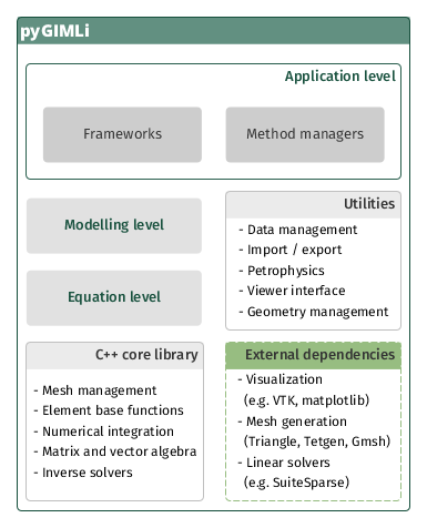
pyGIMLi is organized in three different abstraction levels:

Application level

In the application level, ready-to-use method managers and frameworks are provided. Method managers (pygimli.manager) hold all relevant functionality related to a geophysical method. A method manager can be initialized with a data set and used to analyze and visualize this data set, create a corresponding mesh, and carry out an inversion. Various method managers are available in pygimli.physics. Frameworks (pygimli.frameworks) are generalized abstractions of standard and advanced inversions tasks such as time-lapse or joint inversion for example. Since frameworks communicate through a unified interface, they are method independent.

Modelling level

In the modelling level, users can set up customized forward operators that map discretized parameter distributions to a data vector. Once defined, it is straightforward to set up a corresponding inversion workflow or combine the forward operator with existing ones.

Equation level

The underlying equation level allows to directly access the finite element (pygimli.solver.solveFiniteElements()) and finite volume (pygimli.solver.solveFiniteVolume()) solvers to solve various partial differential equations on unstructured meshes, i.e. to approach various physical problems with possibly complex 2D and 3D geometries.

2.2. Module/method overview

pygimli.physics.em	Frequency-domain (FD) or time-domain (TD) semi-analytical 1D solutions
pygimli.physics.ert	Electrical Resistivity Tomography (ERT)
pygimli.physics.gravimetry	Solve gravimetric and magneto static problems in 2D and 3D analytically
pygimli.physics.petro	Various petrophysical models
pygimli.physics.seismics	Full wave form seismics utilities and simulations
pygimli.physics.SIP	Spectral induced polarization (SIP) measurements and fittings.
pygimli.physics.sNMR	Surface nuclear magnetic resonance (NMR) data inversion
pygimli.physics.traveltime	Refraction seismics or first arrival traveltime calculations.
pygimli.physics.ves	Direct current electromagnetics

method	Forward	Inverse	Dimension
em	✓	✓	1D
ert	✓	✓	2D, 3D, 4D
gravimetry	✓	✓	2D, 3D
magnetics	✓	✓	2D, 3D
petro	✓	✓	dimensionless
seismics	✓	-	“1D”
SIP	✓	✓	1D, 2D
sNMR	✓	✓	1D
traveltime	✓	✓	2D, (3D)
ves	✓	✓	1D

Basic pyGIMLi classes

pygimli.Matrix	alias of RMatrix
pygimli.Vector	alias of RVector
pygimli.SparseMatrix	alias of RSparseMatrix
pygimli.BlockMatrix	alias of RBlockMatrix
pygimli.DataContainer

Note

Please add docstrings for abovementioned classes and then use autosummary function for user guide!

pyGIMLi class	Description
Matrix	All elements are stored column-wise, i.e. all rows A[i] are of type pg.Vector. This matrix is used for storing dense data (like ERT Jacobians) and doing simple algebra.
Vector	One dimensional array aka Vector of limited size to store data, like ERT sensitivities.
SparseMatrix	Used for numerical approximation of partial differential equations like finite-element or finite volume. Not typically used unless efficiency is of importance. It exists also complex-valued as pg.matrix.CSparseMatrix
BlockMatrix	Arbitrary matrices are combined into a logical matrix. This is of importance for inversion frameworks, e.g., concatenated Jacobian matrices during joint inversions.
DataContainer	Data container storing the individual data values as well as any description how they were obtained, e.g. the geometry of source and receivers.

2.3. Viewer interface

In pygimli we provide some basic post-processing routines using the matplotlib visualization framework. The main visualization call is pygimli.viewer.show() which is sufficient for most meshes, fields, models and streamline views. It forwards the object to be plotted to a known visualization function. pygimli.viewer.showMesh() is the typical call for the visualization of 2D data.

However, the underlying show functions only provide an input instance and are not directly responsible for plotting the data. Depending on the data type, pg.viewer.showMesh() then again forwards to the following instances of pg.viewer.mpl:

Data type	Draw function
2D meshes	drawMesh
Value per mesh cell - model patch	drawModel
Value per mesh node - scalar field	drawField
Iterable of type [float,float] - vector field	drawStreams
PosVector - vector field	drawStreams
Pos - sensor position vector	drawSensors

An empty show call creates an empty ax window:

Show code cell source Hide code cell source

import pygimli as pg
import pygimli.meshtools as mt
world = mt.createWorld(start=[-10, 0], end=[10, -10],
                       layers=[-3, -7], worldMarker=True)
mesh = mt.createMesh(world, quality=32, area=0.2, smooth=[1, 10])

res = [[1,10],[2,100],[3,999]]

cell_markers = mesh.cellMarkers()
resistivity = [res[marker-1][1] for marker in cell_markers]
nodeDta = pg.meshtools.cellDataToNodeData(mesh, resistivity)

pg.show()

(<AxesSubplot: >, None)

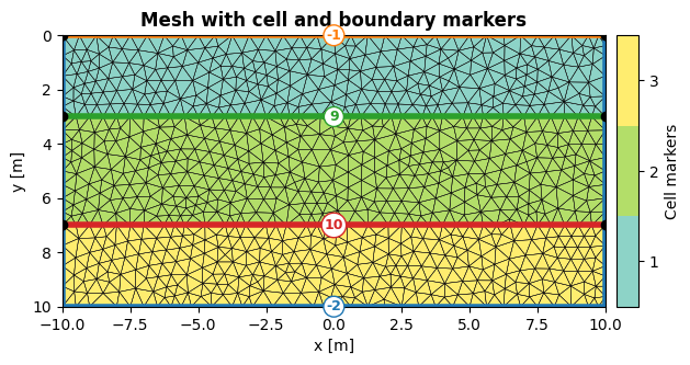
The functions pygimli.viewer.show() and pygimli.viewer.showMesh() return the matplotlib axis object as well as the colorbar object. This allows for further customization of the plot. The following example plots the mesh with cell and boundary markers as “minimal working example”. The orientation of the colorscale can either be parallel to the x- (orientation="horizontal") or y-axis (orientation="vertical"). Further customization of axes or the colorbar can be done by accessing the returned objects directly:

Show code cell source Hide code cell source

ax,cbar = pg.viewer.show(mesh, markers=True, showMesh=True, orientation="vertical")
ax.set_title("Mesh with cell and boundary markers", fontweight="bold")
ax.set_xlabel("x [m]")
ax.set_ylabel("y [m]")

Text(46.972222222222186, 0.5, 'y [m]')

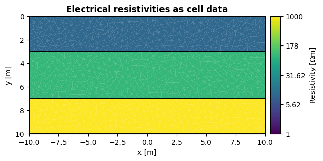
If you want to plot data on top of a mesh, you can use the data argument. The following example shows electrical resistivities as cell data:

Show code cell source Hide code cell source

ax, cbar = pg.viewer.show(mesh, data=res, logScale=True, cMin=1, cMax=1000, orientation="vertical", label="Resistivity [$\Omega$m]")
ax.set_title("Electrical resistivities as cell data", fontweight="bold")
ax.set_xlabel("x [m]")
ax.set_ylabel("y [m]")

Text(46.972222222222186, 0.5, 'y [m]')

If you want to plot node data, this can be done with the same argument data. The following example shows the same electrical resistivities as node data:

Show code cell source Hide code cell source

ax, cbar = pg.viewer.show(mesh, data=nodeDta, logScale=True, cMin=1, cMax=1000, orientation = "vertical", label="Resistivity [$\Omega$m]")
ax.set_title("Electrical resistivities as node data", fontweight="bold")
ax.set_xlabel("x [m]")
ax.set_ylabel("y [m]")

Text(46.972222222222186, 0.5, 'y [m]')

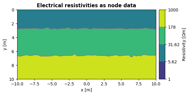
Convert cell to node data

By using the function pg.meshtools.cellDataToNodeData() you can convert cell data to node data. Please refer to the documentation for further details.