pygimli.physics.traveltime

First-arrival traveltime

e.g. refraction or crosshole seismics and GPR

Classes:

• TravelTimeManager

• RefractionNLayer

• DataContainer[TT]

Main entry functions:

• load - load or import from various formats

• createRAData - create refraction data scheme

• simulate - synthetic model computation

• show - show first arrivals as curves or image

Overview

Functions

createCrossholeData([sensors, x, z])	Create crosshole scheme assuming two boreholes with equal sensor numbers.
createGradientModel2D(data, mesh, vTop, vBot)	Create 2D velocity gradient model.
createRAData(sensors[, shotDistance])	Create a refraction data container.
drawFirstPicks(ax, data[, tt, plotva])	Plot first arrivals as lines.
drawTravelTimeData(ax, data[, t])	Draw first arrival traveltime data into mpl ax a.
drawVA(ax, data[, vals, usePos, pseudosection])	Draw apparent velocities as matrix into an axis.
load(fileName[, verbose])	Shortcut to load TravelTime data.
shotReceiverDistances(data[, full])	Distance vector between shot and for each 's' and 'g' in data.
show(data, **kwargs)	Show data.
showVA(data[, usePos, ax])	Show apparent velocity as image plot.
simulate(mesh, scheme[, slowness])	Simulate traveltime measurements.

Classes

DataContainer
DataContainerTT([data])	Data Container for traveltime.
Dijkstra	Dijkstras shortest path finding
Manager
RefractionNLayer([offset, nlay, vbase, verbose])	Forward operator for 1D Refraction seismic with layered model.
RefractionNLayerFix1stLayer([offset, nlay, ...])	FOP for 1D Refraction seismic with layered model (e.g. water layer).
TravelTimeDijkstraModelling(**kwargs)	Forward modelling class for traveltime using Dijktras method.
TravelTimeManager([data])	Manager for refraction seismics (traveltime tomography).
TravelTimeModelling

Functions

pygimli.physics.traveltime.createCrossholeData(sensors=None, x=None, z=None)

Create crosshole scheme assuming two boreholes with equal sensor numbers.

Parameters:

• sensors (array (Nx2)) – Array with position of sensors. Alternatively, specify x and z

• x (iterable [M]) – horizontal positions of boreholes

• z (iterable [M]) – vertical positions of sensors in each borehole

Returns:

scheme – Data container with sensors predefined sensor indices ‘s’ and ‘g’ for shot and receiver numbers.

Return type:

DataContainer

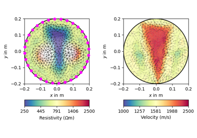
Examples using pygimli.physics.traveltime.createCrossholeData

Crosshole traveltime tomography

Crosshole traveltime tomography

pygimli.physics.traveltime.createGradientModel2D(data, mesh, vTop, vBot, flat=False)

Create 2D velocity gradient model.

Creates a smooth, linear, starting model that takes the slope of the topography into account. This is done by fitting a straight line and using the distance to that as the depth value.

Parameters:

• data (pygimli DataContainer) – The topography list is in here.

• mesh (pygimli.Mesh) – The parametric mesh used for the inversion

• vTop (float) – The velocity at the surface of the mesh

• vBot (float) – The velocity at the bottom of the mesh

Returns:

model – A numpy array with slowness values that can be used to start the inversion.

Return type:

pygimli Vector, length M

pygimli.physics.traveltime.createRAData(sensors, shotDistance=1)

Create a refraction data container.

Default data container for shot and geophon at every sensor position. Predefined sensor indices’s ‘s’ as shot position and ‘g’ as geophon position.

Parameters:

• sensors (ndarray | R3Vector) – Geophon and shot positions (same)

• shotDistances (int [1]) – Distance between shot indices.

Returns:

data – Data container with predefined sensor indices ‘s’ and ‘g’ for shot and receiver numbers.

Return type:

DataContainer

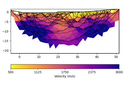
Examples using pygimli.physics.traveltime.createRAData

2D Refraction modelling and inversion

2D Refraction modelling and inversion

Refraction in 3D

Refraction in 3D

Petrophysical joint inversion

Petrophysical joint inversion

Structural coupled cooperative inversion (SCCI)

Structural coupled cooperative inversion (SCCI)

pygimli.physics.traveltime.drawFirstPicks(ax, data, tt=None, plotva=False, **kwargs)

Plot first arrivals as lines.

Parameters:

• ax (matplotlib.axes) – axis to draw the lines in

• data (GIMLI::DataContainer) – data containing shots (“s”), geophones (“g”) and traveltimes (“t”). (:py:class:pygimli.physics.traveltime.DataContainerTT.)

Returns:

gci – list of plotting items (matplotlib lines)

Return type:

list

Examples using pygimli.physics.traveltime.drawFirstPicks

Field data inversion (“Koenigsee”)

Field data inversion ("Koenigsee")

pygimli.physics.traveltime.drawTravelTimeData(ax, data, t=None)

Draw first arrival traveltime data into mpl ax a.

data of type pg.DataContainer must contain sensorIdx ‘s’ and ‘g’ and thus being numbered internally [0..n)

pygimli.physics.traveltime.drawVA(ax, data, vals=None, usePos=True, pseudosection=False, **kwargs)

Draw apparent velocities as matrix into an axis.

Parameters:

• ax (mpl.Axes)

• data (pg.physics.traveltime.DataContainerTT()) – Datacontainer with ‘s’ and ‘g’ Sensorindieces and ‘t’ traveltimes.

• usePos (bool [True]) – Use sensor positions for axes tick labels

• pseudosection (bool [False]) – Show in pseudosection style.

• vals (iterable) – Traveltimes, if None data need to contain ‘t’ values.

pygimli.physics.traveltime.load(fileName, verbose=False, **kwargs)

Shortcut to load TravelTime data.

Import Data and try to assume the file format.

Parameters:

fileName (str)

Returns:

data

Return type:

pg.DataContainer

pygimli.physics.traveltime.shotReceiverDistances(data, full=True)

Distance vector between shot and for each ‘s’ and ‘g’ in data.

Parameters:

• data (pg.DataContainerERT)

• full (bool [True]) – Get distances between shot and receiver position when full is True or only form x coordinate if full is False

Returns:

dists – Array of distances

Return type:

array

pygimli.physics.traveltime.show(data, **kwargs)

Show data.

Examples using pygimli.physics.traveltime.show

2D Refraction modelling and inversion

2D Refraction modelling and inversion

pygimli.physics.traveltime.showVA(data, usePos=True, ax=None, **kwargs)

Show apparent velocity as image plot.

Parameters:

data (pg.DataContainer()) – Datacontainer with ‘s’ and ‘g’ Sensorindieces and ‘t’ traveltimes.

Examples using pygimli.physics.traveltime.showVA

Crosshole traveltime tomography

Crosshole traveltime tomography

Petrophysical joint inversion

Petrophysical joint inversion

pygimli.physics.traveltime.simulate(mesh, scheme, slowness=None, **kwargs)

Simulate traveltime measurements.

Perform the forward task for a given mesh, a slowness distribution (per cell) and return data (traveltime) for a measurement scheme.

Parameters:

• mesh (GIMLI::Mesh) – Mesh to calculate for or use the last known mesh.

• scheme (GIMLI::DataContainer) – Data measurement scheme needs ‘s’ for shot and ‘g’ for geophone data token.

• slowness (array(mesh.cellCount()) | array(N, mesh.cellCount())) –

  Slowness distribution for the given mesh cells can be:

  • a single array of len mesh.cellCount()

  • a matrix of N slowness distributions of len mesh.cellCount()

  • a slowness map [[marker0, slow0], [marker1, slow1], …]

• vel (array(mesh.cellCount()) | array(N, mesh.cellCount())) – Velocity distribution for the mesh cells (overwrites slowness!).

• secNodes (int [2]) – Number of refinement nodes to increase accuracy of the forward calculation.

• noiseLevel (float [0.0]) – Add relative noise to the simulated data. noiseLevel*100 in %

• noiseAbs (float [0.0]) – Add absolute noise to the simulated data in ms.

• seed (int [None]) – Seed the random generator for the noise.

Keyword Arguments:

• returnArray ([False]) – Return only the calculated times.

• verbose ([self.verbose]) – Overwrite verbose level.

• **kwargs – Additional kwargs …

Returns:

t – The resulting simulated travel time values (returnArray=True) or DataContainer containing them in t field (returnArray=False). Either one column array or matrix in case of slowness matrix.

Return type:

array(N, data.size()) | DataContainer

Examples using pygimli.physics.traveltime.simulate

2D Refraction modelling and inversion

2D Refraction modelling and inversion

Crosshole traveltime tomography

Crosshole traveltime tomography

Petrophysical joint inversion

Petrophysical joint inversion

Structural coupled cooperative inversion (SCCI)

Structural coupled cooperative inversion (SCCI)

Classes

pygimli.physics.traveltime.DataContainer

alias of DataContainerTT

class pygimli.physics.traveltime.DataContainerTT(data=None, **kwargs)

Bases: DataContainer

Data Container for traveltime.

__init__(data=None, **kwargs)

Initialize empty data container, load or copy existing.

class pygimli.physics.traveltime.Dijkstra

Bases: instance

Dijkstras shortest path finding

class DistancePair_

Bases: instance

Definition for the priority queue

__init__((object)arg1) → object :

C++ signature :

void* __init__(_object*)

__init__( (object)arg1, (object)f, (object)s) -> object :

C++ signature :

void* __init__(_object*,double,GIMLI::Dijkstra::Edge_ {lvalue})

property first

property second

class Edge_

Bases: instance

__init__((object)arg1) → object :

C++ signature :

void* __init__(_object*)

__init__( (object)arg1, (object)a, (object)b) -> object :

C++ signature :

void* __init__(_object*,unsigned long,unsigned long)

property end

property start

__init__((object)arg1) → object :

C++ signature :

void* __init__(_object*)

__init__( (object)arg1, (object)graph) -> object :

C++ signature :

void* __init__(_object*,std::map<unsigned long, std::map<unsigned long, GIMLI::GraphDistInfo, std::less<unsigned long>, std::allocator<std::pair<unsigned long const, GIMLI::GraphDistInfo> > >, std::less<unsigned long>, std::allocator<std::pair<unsigned long const, std::map<unsigned long, GIMLI::GraphDistInfo, std::less<unsigned long>, std::allocator<std::pair<unsigned long const, GIMLI::GraphDistInfo> > > > > >)

distance((object)arg1, (object)root, (object)node) → object :

Distance from root to node.

C++ signature :

double distance(GIMLI::Dijkstra {lvalue},unsigned long,unsigned long)

distance( (object)arg1, (object)node) -> object :

Distance to node to the last known root.

C++ signature :

double distance(GIMLI::Dijkstra {lvalue},unsigned long)

distances((object)arg1, (object)root) → object :

All distances to root.

C++ signature :

GIMLI::Vector<double> distances(GIMLI::Dijkstra {lvalue},unsigned long)

distances( (object)arg1) -> object :

All distances from to last known root.

C++ signature :

GIMLI::Vector<double> distances(GIMLI::Dijkstra {lvalue})

graph((object)arg1) → object :

C++ signature :

std::map<unsigned long, std::map<unsigned long, GIMLI::GraphDistInfo, std::less<unsigned long>, std::allocator<std::pair<unsigned long const, GIMLI::GraphDistInfo> > >, std::less<unsigned long>, std::allocator<std::pair<unsigned long const, std::map<unsigned long, GIMLI::GraphDistInfo, std::less<unsigned long>, std::allocator<std::pair<unsigned long const, GIMLI::GraphDistInfo> > > > > > {lvalue} graph(GIMLI::Dijkstra {lvalue})

graph( (object)arg1) -> object :

C++ signature :

std::map<unsigned long, std::map<unsigned long, GIMLI::GraphDistInfo, std::less<unsigned long>, std::allocator<std::pair<unsigned long const, GIMLI::GraphDistInfo> > >, std::less<unsigned long>, std::allocator<std::pair<unsigned long const, std::map<unsigned long, GIMLI::GraphDistInfo, std::less<unsigned long>, std::allocator<std::pair<unsigned long const, GIMLI::GraphDistInfo> > > > > > graph(GIMLI::Dijkstra {lvalue})

graphInfo((object)arg1, (object)na, (object)nb) → object :

C++ signature :

GIMLI::GraphDistInfo graphInfo(GIMLI::Dijkstra {lvalue},unsigned long,unsigned long)

setGraph((object)arg1, (object)graph) → object :

C++ signature :

void* setGraph(GIMLI::Dijkstra {lvalue},std::map<unsigned long, std::map<unsigned long, GIMLI::GraphDistInfo, std::less<unsigned long>, std::allocator<std::pair<unsigned long const, GIMLI::GraphDistInfo> > >, std::less<unsigned long>, std::allocator<std::pair<unsigned long const, std::map<unsigned long, GIMLI::GraphDistInfo, std::less<unsigned long>, std::allocator<std::pair<unsigned long const, GIMLI::GraphDistInfo> > > > > >)

setStartNode((object)arg1, (object)startNode) → object :

C++ signature :

void* setStartNode(GIMLI::Dijkstra {lvalue},unsigned long)

shortestPath((object)arg1, (object)start, (object)end) → object :

Get the shortest way from node index start to end.

C++ signature :

GIMLI::Vector<unsigned long> shortestPath(GIMLI::Dijkstra {lvalue},unsigned long,unsigned long)

shortestPathTo((object)arg1, (object)node, (object)way) → object :

Get the shortest way from root to node. Inline version.

C++ signature :

void* shortestPathTo(GIMLI::Dijkstra {lvalue},unsigned long,GIMLI::Vector<unsigned long> {lvalue})

shortestPathTo( (object)arg1, (object)node) -> object :

Get the shortest way from root to node.

C++ signature :

GIMLI::Vector<unsigned long> shortestPathTo(GIMLI::Dijkstra {lvalue},unsigned long)

pygimli.physics.traveltime.Manager

alias of TravelTimeManager

class pygimli.physics.traveltime.RefractionNLayer(offset=0, nlay=3, vbase=1100, verbose=True)

Bases: ModellingBaseMT__

Forward operator for 1D Refraction seismic with layered model.

__init__(offset=0, nlay=3, vbase=1100, verbose=True)

Init forward operator. Model are velocity increases.

Parameters:

• offset (iterable) – vector of offsets between shot and geophone

• nlay (int) – number of layers

• vbase (float) – base velocity (all values are above)

response(model)

Return forward response f(m).

thkVel(model)

Return thickness and velocity vectors from model.

class pygimli.physics.traveltime.RefractionNLayerFix1stLayer(offset=0, nlay=3, v0=1465, d0=200, muteDirect=False, verbose=True)

Bases: ModellingBaseMT__

FOP for 1D Refraction seismic with layered model (e.g. water layer).

__init__(offset=0, nlay=3, v0=1465, d0=200, muteDirect=False, verbose=True)

Init forward operator for velocity increases with fixed 1st layer.

Parameters:

• offset (iterable) – vector of offsets between shot and geophone

• nlay (int) – number of layers

• v0 (float) – First layer velocity (at the same time base velocity)

• d0 (float) – Depth of first layer in meter.

• muteDirect (bool [False]) – Mute the direct arrivals from the first layer.

response(model)

Return forward response f(m).

thkVel(model)

Return thickness and velocity vectors from model.

class pygimli.physics.traveltime.TravelTimeDijkstraModelling(**kwargs)

Bases: MeshModelling

Forward modelling class for traveltime using Dijktras method.

__init__(**kwargs)

Initialize.

Variables:

• fop (pg.frameworks.Modelling)

• data (pg.DataContainer)

• modelTrans ([pg.trans.TransLog()])

Keyword Arguments:

**kwargs – fop: Modelling

createGraph(slowness)

Create Dijkstra graph.

createJacobian(par)

Create Jacobian (way matrix).

createRefinedFwdMesh(mesh)

Refine the current mesh for higher accuracy.

This is called automatic when accessing self.mesh() so it ensures any effect of changing region properties (background, single).

createStartModel(dataVals)

Create a starting model from data values (gradient or constant).

property dijkstra

Return current Dijkstra graph associated to mesh and model.

drawData(ax, data=None, **kwargs)

Draw the data (as apparent velocity crossplot by default).

Parameters:

data (pg.DataContainer)

drawModel(ax, model, **kwargs)

Draw the model.

response(par)

Return forward response (simulated traveltimes).

setDataPost(data)

Set data after forward operator has been initialized.

setMeshPost(mesh)

Set mesh after forward operator has been initialized.

way(s, g)

Return node indices for the way from the shot to the receiver.

The index is based on the given data, mesh and last known model.

class pygimli.physics.traveltime.TravelTimeManager(data=None, **kwargs)

Bases: MeshMethodManager

Manager for refraction seismics (traveltime tomography).

TODO Document main members and use default MethodManager interface e.g., self.inv, self.fop, self.paraDomain, self.mesh, self.data

__init__(data=None, **kwargs)

Create an instance of the Traveltime manager.

Parameters:

data (GIMLI::DataContainer | str) – You can initialize the Manager with data or give them a dataset when calling the inversion.

applyMesh(mesh, secNodes=None, ignoreRegionManager=False)

Apply mesh, i.e. set mesh in the forward operator class.

checkData(data)

Return data from container.

checkError(err, dataVals)

Return relative error.

createForwardOperator(**kwargs)

Create default forward operator for Traveltime modelling.

Your want your Manager use a special forward operator you can add them here on default Dijkstra is used.

createMeshMovedToMeshManager(data=None, **kwargs)

Create default inversion mesh.

Inversion mesh for traveltime inversion does not need boundary region.

Parameters:

data (DataContainer) – Data container to read sensors from.

Keyword Arguments:

` (Forwarded to)

createTraveltimefield(v=None, startPos=None, withSec=False)

Compute a single traveltime field.

drawRayPaths(ax, model=None, rayPaths=None, **kwargs)

Draw the the ray paths for model or last model.

If model is not specified, the last calculated Jacobian is used.

Parameters:

• rayPaths (list of np.array) – x/y column array with ray point positions

• model (array) – Velocity model for which to calculate and visualize ray paths (the default is model for last Jacobian calculation in self.velocity).

• ax (matplotlib.axes object) – To draw the model and the path into.

• **kwargs (type) – Additional arguments passed to LineCollection (alpha, linewidths, color, linestyles).

Returns:

lc

Return type:

matplotlib.LineCollection

getRayPaths(model=None)

Compute ray paths.

If model is not specified, the last calculated Jacobian is used.

Parameters:

model (array) – Velocity model for which to calculate and visualize ray paths (the default is model for last Jacobian calculation in self.velocity).

Return type:

list of two-column array holding x and y positions

invert(data=None, useGradient=True, vTop=500, vBottom=5000, secNodes=None, **kwargs)

Invert data.

Parameters:

• data (pg.DataContainer()) – Data container with at least SensorIndices ‘s g’ (shot/geophone) & data values ‘t’ (traveltime in s) and ‘err’ (absolute error in s)

• useGradient (bool [True]) – Use gradient starting model typical for refraction cases. For crosshole tomography geometry you should set this to False for a non-gradient (e.g. homogeneous) starting model.

• vTop (float) – Top velocity for gradient starting model.

• vBottom (float) – Bottom velocity for gradient starting model.

• secNodes (int [2]) – Number of secondary nodes for accuracy of forward computation.

Returns:

Mapped (for paradomain) velocity model.

Return type:

model

Keyword Arguments:

kwargs (**) – Inversion related arguments: See pygimli.frameworks.MeshMethodManager.invert

load(fileName)

Load any supported data file.

rayCoverage()

Ray coverage, i.e. summed raypath lengths.

saveResult(folder=None, size=(16, 10), verbose=False, **kwargs)

Save the results in a specified (or date-time derived) folder.

Saved items are:

• Resulting inversion model

• Velocity vector

• Coverage vector

• Standardized coverage vector

• Mesh (bms and vtk with results)

Parameters:

• path (str[None]) – Path to save into. If not set the name is automatically created

• size ((float, float) (16,10)) – Figure size.

Keyword Arguments:

showResults (Will be forwarded to)

Returns:

Name of the result path.

Return type:

str

showCoverage(ax=None, name='coverage', **kwargs)

Show the ray coverage in log-scale.

showFit(axs=None, firstPicks=True, **kwargs)

Show data fit as first-break picks or apparent velocity.

showMisfit()

Show data misfit (traveltime) color-coded.

showRayPaths(model=None, ax=None, **kwargs)

Show the model with ray paths for given model.

If not model specified, the last calculated Jacobian is taken.

Parameters:

• model (array) – Velocity model for which to calculate and visualize ray paths (the default is model for last Jacobian calculation in self.velocity).

• ax (matplotlib.axes object) – To draw the model and the path into.

• **kwargs (type) – forward to drawRayPaths

Returns:

• ax (matplotlib.axes object)

• cb (matplotlib.colorbar object (only if model is provided))

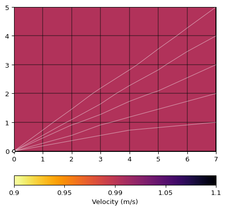
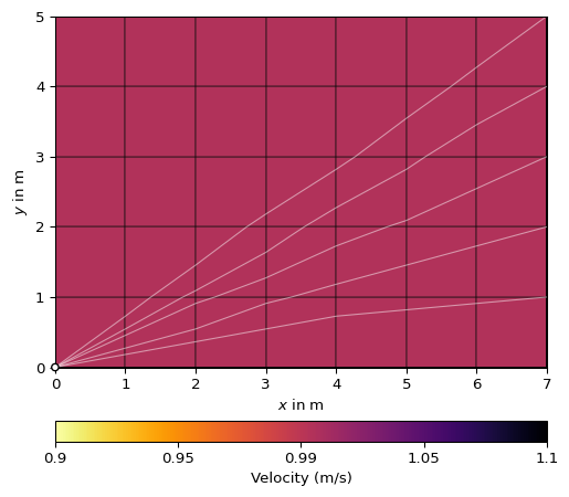
Examples

>>> import pygimli as pg
>>> from pygimli.physics import traveltime as tt
>>>
>>> x, y = 8, 6
>>> mesh = pg.createGrid(x, y)
>>> data = tt.createRAData([(0, 0)] + [(x, i) for i in range(y)],
...                       shotDistance=y+1)
>>> data["t"] = 1.0
>>> mgr = tt.Manager(data)
>>> mgr.applyMesh(mesh, secNodes=10)
>>> ax, cb = mgr.showRayPaths(showMesh=True, diam=0.1)

(png, pdf)

simulate(mesh=None, scheme=None, slowness=None, vel=None, seed=None, secNodes=2, noiseLevel=0.0, noiseAbs=0.0, **kwargs)

Simulate traveltime measurements.

Perform the forward task for a given mesh, a slowness distribution (per cell) and return data (traveltime) for a measurement scheme.

Parameters:

• mesh (GIMLI::Mesh) – Mesh to calculate for or use the last known mesh.

• scheme (GIMLI::DataContainer) – Data measurement scheme needs ‘s’ for shot and ‘g’ for geophone data token.

• slowness (array(mesh.cellCount()) | array(N, mesh.cellCount())) –

  Slowness distribution for the given mesh cells can be:

  • a single array of len mesh.cellCount()

  • a matrix of N slowness distributions of len mesh.cellCount()

  • a slowness map [[marker0, slow0], [marker1, slow1], …]

• vel (array(mesh.cellCount()) | array(N, mesh.cellCount())) – Velocity distribution for the mesh cells (overwrites slowness!).

• secNodes (int [2]) – Number of refinement nodes to increase accuracy of the forward calculation.

• noiseLevel (float [0.0]) – Add relative noise to the simulated data. noiseLevel*100 in %

• noiseAbs (float [0.0]) – Add absolute noise to the simulated data in ms.

• seed (int [None]) – Seed the random generator for the noise.

Keyword Arguments:

• returnArray ([False]) – Return only the calculated times.

• verbose ([self.verbose]) – Overwrite verbose level.

• **kwargs – Additional kwargs …

Returns:

t – The resulting simulated travel time values (returnArray=True) or DataContainer containing them in t field (returnArray=False). Either one column array or matrix in case of slowness matrix.

Return type:

array(N, data.size()) | DataContainer

standardizedCoverage()

Standardized coverage vector (0|1) using neighbor info.

property velocity

Return velocity vector (the inversion model).

pygimli.physics.traveltime.TravelTimeModelling

alias of TravelTimeDijkstraModelling