Note
Go to the end to download the full example code.
Regularization - concepts explained#
In geophysical inversion, we minimize the data objective functional as the L2 norm of the misfit between data \(d\) and the forward response \(f(m)\) of the model \(m\), weighted by the data error \(\epsilon\):
As this minimization problem is non-unique and ill-posed, we introduce a regularization term \(\Phi\), weighted by a regularization parameter \(\lambda\):
The regularization strength \(\lambda\) should be chosen so that the data are fitted within noise, i.e. \(\chi^2=\Phi_d/N=1\).
In the term \(\Phi_m\) we put our expectations to the model, e.g. to be close to any prior model. In many cases we do not have much information and aim for the smoothest model that is able to fit our data. We describe it by the operator \(W_m\):
The regularization operator is defined by some constraint operator \(C\) weighted by some weighting function \(w\) so that \(W_m=\mbox{diag}(w) C\). The operator \(C\) can be a discrete smoothness operator, or the identity to keep the model close to the reference model \(m_{ref}\).
We start with importing the numpy, matplotlib and pygimli libraries
import numpy as np
import matplotlib.pyplot as plt
import pygimli as pg
import pygimli.meshtools as mt
Regularization drives the model where the data are too weak to constrain the model. In order to explain different kinds of regularization (also called constraints), we use a very simple mapping forward operator: The values at certain positions are picked.
from pygimli.frameworks import PriorModelling
Implementation#
determine the indices where the cells are
ind = [mesh.findCell(po).id() for po in pos]
forward response: take the model at indices
response = model[ind]
Jacobian matrix
J = pg.SparseMapMatrix()
J.resize(len(ind), mesh.cellCount())
for i, n in enumerate(self.ind):
    self.J.setVal(i, n, 1.0)
We exemplify this on behalf of a simple triangular mesh in a rectangular domain.
rect = mt.createRectangle(start=[0, -10], end=[10, 0])
mesh = mt.createMesh(rect, quality=34.5, area=0.3)
print(mesh)
Mesh: Nodes: 377 Cells: 684 Boundaries: 1060
We define two positions where we associate two arbitrary values.
We set up an inversion instance with the forward operator and prepare the keywords for running the inversion always the same way: - the data vector - the error vector (as relative error) - a starting model value (could also be vector)
Classical smoothness constraints#
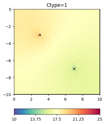
We will have a closer look at the regularization matrix \(C`\).
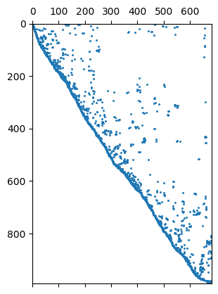
992 684 Mesh: Nodes: 377 Cells: 684 Boundaries: 1060
[ 48 116] 2 [1.0, -1.0]
How does that change the regularization matrix \(C\)?
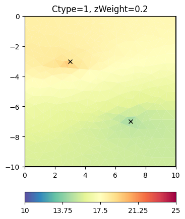
0.19999999999999996 1.0
Now we try some other regularization options.
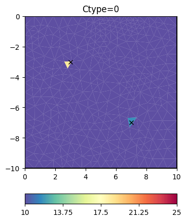
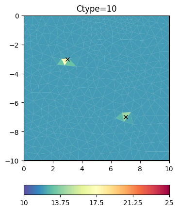
Obviously, the damping keeps the model small (log 1=0) as the starting model is NOT a reference model by default. We enable this by specifying the isReference switch.
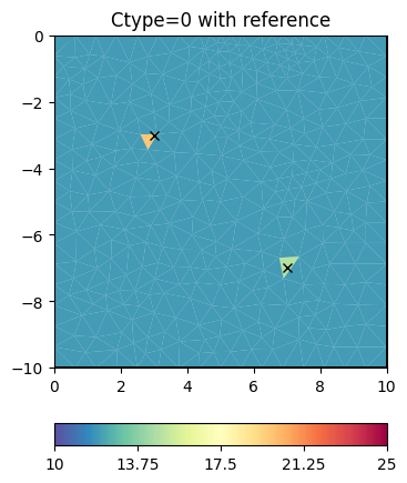
cType=10 means a mix between 1st order smoothness (1) and damping (0)
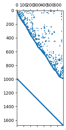
In the matrix both contributions are under each other
1676 684
Mesh: Nodes: 377 Cells: 684 Boundaries: 1060
We see that we have the first order smoothness and the identity matrix
below each other. We can also use a second-order (-1 2 -1) smoothness
operator by cType=2.
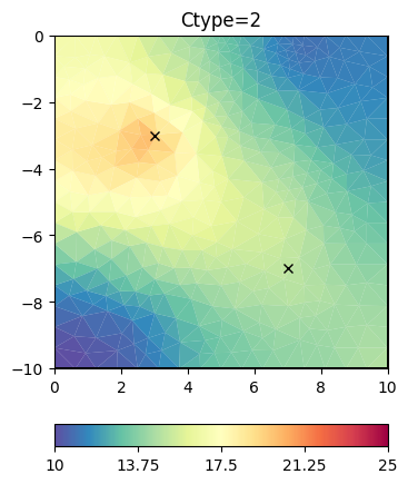
We have a closer look at the constraints matrix
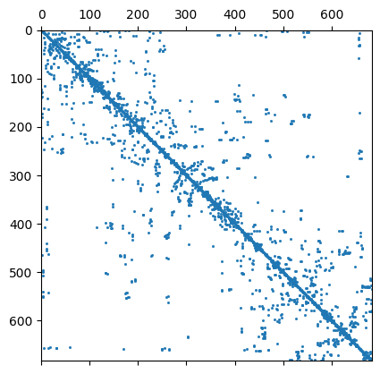
684 684 Mesh: Nodes: 377 Cells: 684 Boundaries: 1060
It looks like a Laplace operator and seems to have a wider range compared to first-order smoothness.
Geostatistical regularization#
The idea is that not only neighbors are correlated to each other but to have a wider correlation by using an operator
More details can be found in https://www.pygimli.org/_tutorials_auto/3_inversion/plot_6-geostatConstraints.html
Application#
We can pass the correlation length directly to the inversion instance
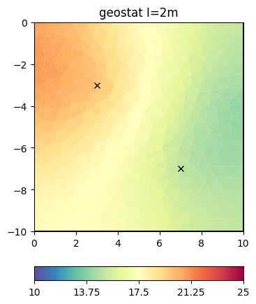
This look structurally similar to the second-order smoothness, but can drive values outside the expected range in regions of no data coverage. We change the correlation lengths and the dip to be inclining
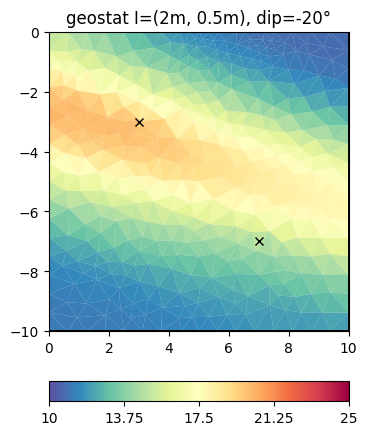
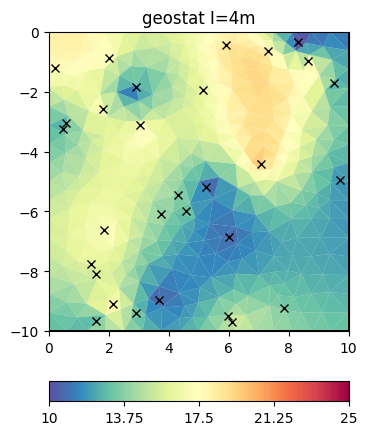
We now add many more points.
np.random.seed(42) # reproducabilty is our friend
N = 30
x = np.random.rand(N) * 10
y = -np.random.rand(N) * 10
v = np.random.rand(N) * 10 + 10
and repeat the above computations
pos = [pg.Pos(xi, yi) for xi, yi in zip(x, y)]
fop = PriorModelling(mesh, pos)
inv = pg.Inversion(fop=fop, verbose=True)
inv.setRegularization(correlationLengths=[4, 4])
result = inv.run(v, relativeError=0.03, startModel=10, lam=10)
ax, _ = pg.show(mesh, result, **plotkw)
out = ax.plot(x, y, "kx")
t = ax.set_title("geostat I=4m")
--------------------------------------------------------------------------------
--------------------------------------------------------------------------------
inv.iter 1 ... --------------------------------------------------------------------------------
inv.iter 2 ... --------------------------------------------------------------------------------
inv.iter 3 ... ################################################################################
#                Abort criterion reached: dPhi = 0.02 (< 2.0%)                 #
################################################################################
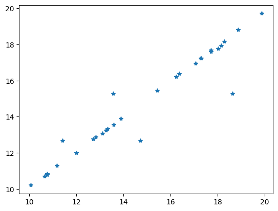
Comparing the data with the model response is always a good idea.
Individual regularization operators#
Say you want to combine geostatistic operators with a damping, you can create a block matrix pasting the matrix vertically.
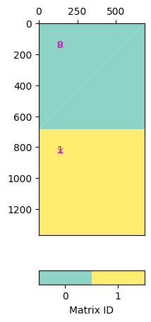
Note that in pg.matrix you find a lot of matrices and matrix generators.
We set this matrix directly and do the inversion.
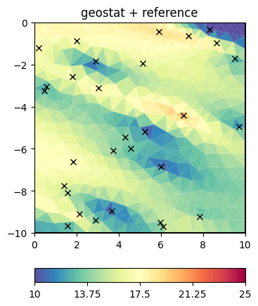
--------------------------------------------------------------------------------
--------------------------------------------------------------------------------
inv.iter 1 ... --------------------------------------------------------------------------------
inv.iter 2 ... --------------------------------------------------------------------------------
inv.iter 3 ... ################################################################################
#                Abort criterion reached: dPhi = 0.11 (< 2.0%)                 #
################################################################################
If you are using a method manager, you access the inversion instance by mgr.inv and the forward operator by mgr.fop.
Note
Take-away messages
regularization drives the model where data are weak
think and play with your assumptions to the model
there are several predefined options
geostatistical regularization can be superior, because: - it is mesh-independent - it better fills the data gaps (e.g. 3D inversion of 2D profiles)