Note
Go to the end to download the full example code or to run this example in your browser via Binder.
ERT inversion of data measured on a standing tree#
This example is about inversion of ERT data around a hollow lime tree. It applies the BERT methodology of Günther et al. (2006) to trees, first documented by Göcke et al. (2008) and Martin & Günther (2013). It has already been used in the BERT tutorial (Günther & Rücker, 2009-2023) in chapter 3.3 (closed geometries).
generate circular geometry
geometric factor generation
circular data representation
inversion
import pygimli as pg
import pygimli.meshtools as mt
from pygimli.physics import ert
Get some example data with, typically by a call like data = ert.load(“filename.dat”)
data = pg.getExampleData('ert/hollow_limetree.ohm', verbose=True)
print(data)
[:::::::::::::::::::::::::::::::::::: 100% ::::::::::::::::::::::::::::::::::::] 7760 of 7760 complete
md5: 51bd5f8be795918098a64cc75795409d
Data: Sensors: 24 data: 264, nonzero entries: ['a', 'b', 'i', 'm', 'n', 'r', 'u', 'valid']
It uses 24 electrodes around the circumference and applies a dipole-dipole (AB-MN) array. For each of the 24 dipoles being used as current injection (AB), 21 potential dipoles (from 3-4 to 23-24) can be measured of which 10 are measured, so that we end up in a total of 24*11=264 measurements. Apart from current (‘a’ and ‘b’) and potential (‘m’, ‘n’) electrodes, the file contains current (‘i’), voltage (‘u’) and resistance (‘r’) vectors for each of the 264 data.
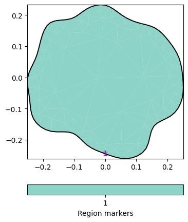
We first generate the geometry by creating a closed polygon. Between each two electrodes, we place three additional nodes whose positions are interpolated using a spline.
plc = mt.createPolygon(data.sensors(), isClosed=True,
                       addNodes=3, interpolate='spline')
ax, cb = pg.show(plc)
From this geometry, we create a triangular mesh with a quality factor, a maximum triangle area and post-smoothing.
mesh = mt.createMesh(plc, quality=34.3, area=2e-4, smooth=[10, 1])
print(mesh)
ax, _ = pg.show(mesh)
for i, s in enumerate(data.sensors()):
    ax.text(s.x(), s.y(), str(i+1), zorder=100)
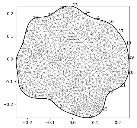
Mesh: Nodes: 917 Cells: 1732 Boundaries: 2648
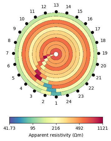
We first create the geometric factors to multiply the resistances to obtain “mean” resistivities for every quadrupol. We do this numerically using a refined mesh with quadratic shape functions using a constant resistivity of 1. The inverse of the modelled resistances is the geometric factor so that all apparent resistivities become 1. We then generate apparent resistivity, store it in the data and show it.
data["k"] = ert.createGeometricFactors(data, mesh=mesh, numerical=True)
data["rhoa"] = data["r"] * data["k"]
ax, cb = ert.show(data, "rhoa", circular=True)
/home/florian/actions-runner/_work/pyGIMLi/pyGIMLi/source/pygimli/physics/ert/visualization.py:353: RuntimeWarning: invalid value encountered in cast
  ne = np.array(xe/de, dtype=int)
Note that we use the option circular. The values have almost rotation symmetry with lower values for shallow penetrations and higher ones for larger current-voltage distances.
We estimate a measuring error using default values (3%) and feed it into the ERT Manager.
data.estimateError()
mgr = ert.Manager(data)
mgr.invert(mesh=mesh, verbose=True)
--------------------------------------------------------------------------------
--------------------------------------------------------------------------------
inv.iter 1 ... --------------------------------------------------------------------------------
inv.iter 2 ... --------------------------------------------------------------------------------
inv.iter 3 ... --------------------------------------------------------------------------------
inv.iter 4 ... ################################################################################
#                Abort criterion reached: dPhi = 0.51 (< 2.0%)                 #
################################################################################

1732 [199.6627189443874,...,285.9117592975968]
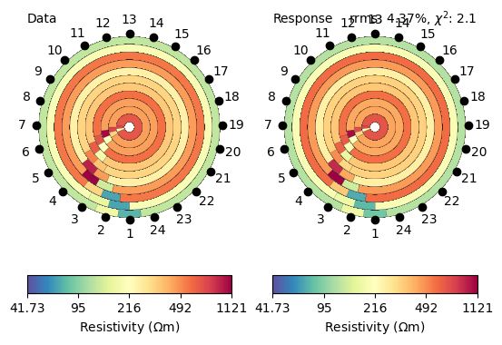
We achieve a fairly good data fit with a chi-square value of 2 and compare data and model response, both are looking very similar.
ax = mgr.showFit(circular=True)
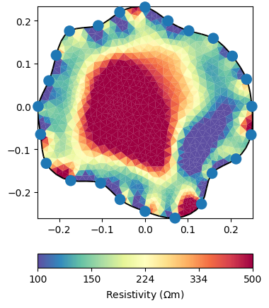
Finally, we have a look at the resulting resistivity distribution. It clearly shows a cavity inside the tree trunk, indicated by the high resistivity region.
ax, cb = mgr.showResult(cMin=100, cMax=500, coverage=1)
References#
Günther, T., Rücker, C. & Spitzer, K. (2006): Three-dimensional modeling & inversion of dc resistivity data incorporating topography – II: Inversion. Geophys. J. Int. 166, 506-517, doi:10.1111/j.1365-246X.2006.03011.x
Göcke, L., Rust, S., Weihs, U., Günther, T. & Rücker, C. (2008): Combining sonic and electrical impedance tomography for the nondestructive testing of trees. - Western Arborist, Spring/2008: 1-11.
Martin, T. & Günther, T. (2013): Complex Resistivity Tomography (CRT) for fungus detection on standing oak trees. European Journal of Forest Research 132(5), 765-776, doi:10.1007/s10342-013-0711-4
Total running time of the script: (0 minutes 17.850 seconds)