# Checkout www.pygimli.org for more examples

Raypaths in layered and gradient models

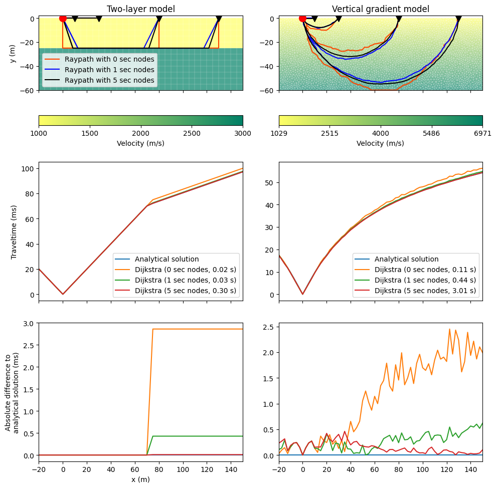
This example performs raytracing for a two-layer and a vertical gradient model and compares the resulting traveltimes to existing analytical solutions. An approximation of the raypath is found by finding the shortest-path through a grid of nodes. The possible angular coverage is small when only corner points of a cell (primary nodes) are used for this purpose. The angular coverage, and hence the numerical accuracy of traveltime calculations, can be significantly improved by a few secondary nodes along the cell edges. Details can be found in Giroux & Larouche (2013).

from math import asin, tan

import matplotlib.pyplot as plt
import numpy as np
import pygimli as pg
import pygimli.meshtools as mt
from pygimli.viewer.mpl import drawMesh

from pygimli.physics import TravelTimeManager

Two-layer model

We start by building a regular grid.

mesh_layered = mt.createGrid(
    np.arange(-20, 155, step=5, dtype=float), np.linspace(-60, 0, 13))

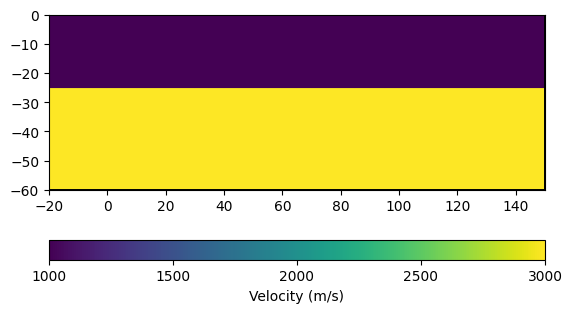
We now construct the velocity vector for the two-layer case by iterating over the cells. Cells above 25 m depth are assigned \(v = 1000\) m/s and cells below are assigned \(v = 3000\) m/s.

vel_layered = np.zeros(mesh_layered.cellCount())
for cell in mesh_layered.cells():
    if cell.center().y() < -25:
        vel = 3000.0
    else:
        vel = 1000.0
    vel_layered[cell.id()] = vel

ax, cb = pg.show(mesh_layered, vel_layered, label="Velocity (m/s)")

We now define the analytical solution. The traveltime at a given offset x is the minimum of the direct and critically refracted wave, where the latter is governed by Snell’s law.

def analyticalSolution2Layer(x, zlay=25, v1=1000, v2=3000):
    """Analytical solution for 2 layer case."""
    tdirect = np.abs(x) / v1  # direct wave
    alfa = asin(v1 / v2)  # critically refracted wave angle
    xreflec = tan(alfa) * zlay * 2.  # first critically refracted
    trefrac = (x - xreflec) / v2 + xreflec * v2 / v1**2
    return np.minimum(tdirect, trefrac)

Vertical gradient model

We first create an unstructured mesh:

sensors = np.arange(131, step=10.0)
plc = mt.createWorld([-20, -60], [150, 0], worldMarker=False)
for pos in sensors:
    plc.createNode([pos, 0.0])
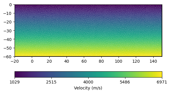
mesh_gradient = mt.createMesh(plc, quality=33, area=3)

A vertical gradient model, i.e. \(v(z) = a + bz\), is defined per cell.

a = 1000
b = 100

vel_gradient = []
for node in mesh_gradient.nodes():
    vel_gradient.append(a + b * abs(node.y()))
vel_gradient = pg.meshtools.nodeDataToCellData(mesh_gradient,
                                               np.array(vel_gradient))
ax, cb = pg.show(mesh_gradient, vel_gradient, label="Velocity (m/s)")

The traveltime for a gradient velocity model is given by:

(1)\[\begin{align}v = \left|b^{-1}cosh^{-1}\left(1 + \frac{b^2 x^2}{2a^2}\right)\right|\end{align}\]

def analyticalSolutionGradient(x, a=1000, b=100):
    """Analytical solution for gradient model."""
    tdirect = np.abs(x) / a  # direct wave
    tmp = 1 + ((b**2 * np.abs(x)**2) / (2 * a**2))
    trefrac = np.abs(b**-1 * np.arccosh(tmp))
    return np.minimum(tdirect, trefrac)

The loop below calculates the travel times and makes the comparison plot.

fig, ax = plt.subplots(3, 2, figsize=(10, 10), sharex=True)

for j, (case, mesh, vel) in enumerate(zip(["layered", "gradient"],
                                          [mesh_layered, mesh_gradient],
                                          [vel_layered, vel_gradient])):
    pg.boxprint(case)
    if case == "gradient":
        ana = analyticalSolutionGradient
    elif case == "layered":
        ana = analyticalSolution2Layer
    for boundary in mesh.boundaries():
        boundary.setMarker(0)

    xmin, xmax = mesh.xmin(), mesh.xmax()
    mesh.createNeighborInfos()

    # In order to use the Dijkstra, we extract the surface positions >0
    mx = pg.x(mesh)
    my = pg.y(mesh)
    px = np.sort(mx[my == 0.0])

    # A data container with index arrays named s (shot) and g (geophones) is
    # created and filled with the positions and shot/geophone indices.
    data = pg.DataContainer()
    data.registerSensorIndex('s')
    data.registerSensorIndex('g')

    for i, pxi in enumerate(px):
        data.createSensor([pxi, 0.0])
        if pxi == 0.0:
            source = i

    nData = len(px)
    data.resize(nData)
    data['s'] = [source] * nData # only one shot at first sensor
    data['g'] = range(nData)  # and all sensors are receiver geophones

    # Draw initial mesh with velocity distribution
    pg.show(mesh, vel, ax=ax[0, j], label="Velocity (m/s)", hold=True,
            logScale=False, cMap="summer_r", coverage=0.7)
    drawMesh(ax[0, j], mesh, color="white", lw=0.21)

    # We compare the accuracy for 0-5 secondary nodes
    sec_nodes = [0, 1, 5]
    t_all = []
    durations = []
    paths = []

    mgr = TravelTimeManager()

    cols = ["orangered", "blue", "black"]
    recs = [1, 3, 8, 13]

    for i, n in enumerate(sec_nodes):

        # Perform traveltime calculations and log time with pg.tic() & pg.toc()
        pg.tic()
        res = mgr.simulate(vel=vel, scheme=data, mesh=mesh, secNodes=n)
        # We need to copy res['t'] here because res['t'] is a reference to
        # an array in res, and res will be removed in the next iteration.
        # Unfortunately, we don't have any reverence counting for core objects yet.
        t_all.append(res['t'].array())
        durations.append(pg.dur())
        pg.toc("Raytracing with %d secondary nodes:" % n)

        for r, p in enumerate(recs):
            if r == 0:
                lab = "Raypath with %d sec nodes" % n
            else:
                lab = None

            recNode = mgr.fop.mesh().findNearestNode([sensors[p], 0.0])
            sourceNode = mgr.fop.mesh().findNearestNode([0.0, 0.0])

            path = mgr.fop.dijkstra.shortestPath(sourceNode, recNode)
            points = mgr.fop.mesh().positions(withSecNodes=True)[path].array()
            ax[0, j].plot(points[:,0], points[:,1], cols[i], label=lab)

    t_ana = ana(px)

    # Upper subplot
    ax[1, j].plot(px, t_ana * 1000, label="Analytical solution")

    for i, n in enumerate(sec_nodes):
        ax[1, j].plot(px, t_all[i] * 1000,
                      label="Dijkstra (%d sec nodes, %.2f s)" % (n, durations[i]))

    ax[2, j].plot(px, np.zeros_like(px), label="Zero line")  # to keep color cycle

    for i, n in enumerate(sec_nodes):
        ax[2, j].plot(px, np.abs(t_all[i] - t_ana) * 1000)

    ax[1, j].legend()

    # Draw sensor positions for the selected receivers
    for p in recs:
        ax[0, j].plot(sensors[p], 0.0, "kv", ms=10)
    ax[0, j].plot(0.0, 0.0, "ro", ms=10)
    ax[0, j].set_ylim(mesh.ymin(), 2)

ax[0, 0].set_title("Two-layer model")
ax[0, 1].set_title("Vertical gradient model")
ax[0, 0].legend()
ax[0, 0].set_ylabel("y (m)")
ax[1, 0].set_ylabel("Traveltime (ms)")
ax[2, 0].set_ylabel("Absolute difference to\nanalytical solution (ms)")
ax[2, 0].set_xlabel("x (m)")
fig.tight_layout()